- CFD, Fluid Flow, FEA, Heat/Mass Transfer
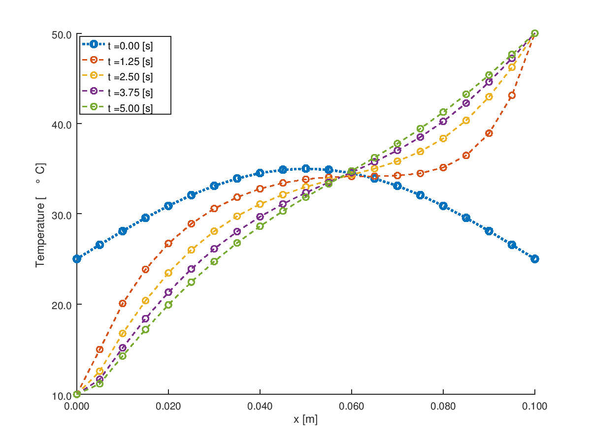
Transient Conduction - 1D
Octave Script
Transient Conduction
OCTAVE is a free program highly compatible to MATLAB. It is a handy tool to solve differential equations numerically with built-in feature or use numerical methods dealing with inversion of matrices. A graphical plot of the results can be generated with ease.
The purpose of this calculation approach is to demonstrate the numerical technique and TDMA (Tri-Diagomal Matrix Algorithm) method to solve transient conduction. Various improvisation is possible in this script such as implementation of Heat Flux and Convective boundaries at the tip, incorporating variable cross-section area such as tapered rod and so on.
Temperature Time History Plots
% Solve 1D heat equation with Backward Time Centre Space scheme
%   d^2T     1      dT
%   ---- = ----- * ----
%   dx^2   alpha    dt
%
  clear; clc;

% L        = length of the domain [m]
  L        = 0.1;
% NN       = number of mesh nodes [number]
  NN       = 21;

% nTime    = number of steps  [number], delta_t = tMax / nTime
  nTime    = 4;
% tMax     = maximum time for the simulation [s]
  tMax     = 5.0;

% alpha    = diffusion coefficient [m^2/s]
% Thermal conductivity [W/m.K]
  k        = 150;
% Density [kg/m^3]
  rho      = 2700;
% Specific heat capacity [J/kg.K]
  Cp       = 450;
  alpha    = k/rho/Cp;

% Specify initial conditions
  dx  = L / (NN - 1);
  x   = [0 : dx: L];
  phi = 25 + 10 * sin(pi .* x / L);
% Specify boundary conditions
  phi0     = 10;
  phiL     = 50;

  dt = tMax / nTime;

% Check for Courant number for numerical stability and bounded solution
  CoNum = alpha * dt / dx^2;
  %If (CoNum >= 2.0)
  %  N = L / ((alpha * dt / 2.0)^0.5);
  %	 NN = round(N);
  %  dx = L / (NN - 1);
  %endif

% --- Coefficients of the Tri-Diagonal System

% T^n(i-1) - 2T^n(i) + T^n(i+1)     1      T^n - T^[n-1](i)
% ----------------------------- = ----- *  --------------
%             dx^2                alpha         dt
%                     .--              --.
%   alpha             |  1     2*alpha   |          alpha            T^[n-1](i)
% - ----- T^n(i-1) +  | --- -  -------   |T^n(i) -  -----T^n(i+1) =  ----------
%    dx^2             |  dt     dx^2     |           dx^2                dt
%                     |__              __|
%
% -  C * T^n(i-1) +         A *          T^n(i) - B *   T^n(i+1) = d(i),  i = 1 ... NN
%
%  A* T^n(i) = B(i) * T(i+1) + C(i) * T(i-1) + d(i), i = 1 ... NN

% subdiagonal C: coefficients of phi(i-1)
  B = (alpha/dx^2) * ones(NN,1);

% superdiagonal B: coefficients of phi(i+1)
  C = B;

% diagonal A: coefficients of phi(i)
  A = (1/dt) * ones(NN, 1) + 2 * B;

% constant term d
  d = zeros(NN, 1);

% Plot temperature profile at t = 0 [s]
  hold on;
  plot(x, phi, "linestyle", ":", "linewidth", 2, "marker", "o");

  for m = 1:nTime
    % Tridiagonal Matrix Algorithm [Ref: S. V. Patankar]
    % If T(1) is specified
	A(1) = 1;     B(1) = 0;

	% Since T(0) and T(NN+1) have no significance
	B(end) = 0;     C(1) = 0;

	d(1) = phi0 / dt;

	P(1) = B(1) / A(1);
    Q(1) = d(1) / A(1);
    for i = 2: NN
      d(i) = phi(i) / dt;
	  P(i) = B(i) / (A(i) - C(i) * P(i-1));
      Q(i) = (d(i) + C(i) * Q(i-1)) / (A(i) - C(i) * P(i-1));
    end
	phi(NN) = phiL;

    % --- Backward substitution
    for i = NN-1 : -1 : 2
      phi(i) = P(i) * phi(i+1) + Q(i);
    end
	phi(1) = phi0;

    plot(x, phi, "linestyle", "--", "linewidth", 1, "marker", "o");
  end

  xlabel('x [m]');  	ylabel('Temperature [\deg C]');
  %grid on; set (gca, "ygrid", "on");

% Format X-axis ticks
  xtick = get (gca, "xtick");
  xticklabel = strsplit (sprintf ("%.3f\n", xtick), "\n", true);
  set (gca, "xticklabel", xticklabel)

% Format Y-Axis ticks
  ytick = get (gca, "ytick");
  yticklabel = strsplit (sprintf ("%.1f\n", ytick), "\n", true);
  set (gca, "yticklabel", yticklabel);

  legengTxt = cell(nTime+1, 1);
  for m = 0: nTime
    legendTxt{m+1} = strcat('t = ', num2str(m * dt, '%.2f'), ' [s]');
  end
  legend(legendTxt, "location", 'northwest');
  hold off;
  print -dpng transCondOneD.png -color -landscape;
The content on CFDyna.com is being constantly refined and improvised with on-the-job experience, testing, and training. Examples might be simplified to improve insight into the physics and basic understanding. Linked pages, articles, references, and examples are constantly reviewed to reduce errors, but we cannot warrant full correctness of all content.
Copyright © 2017 - All Rights Reserved - CFDyna.com
Template by OS Templates