- CFD, Fluid Flow, FEA, Heat/Mass Transfer: Open-source Tools
Combustion Simulation in OpenFOAM
Combustion Simulation in OpenFOAM
Combustion Modeling - Theory and Numerical Simulation
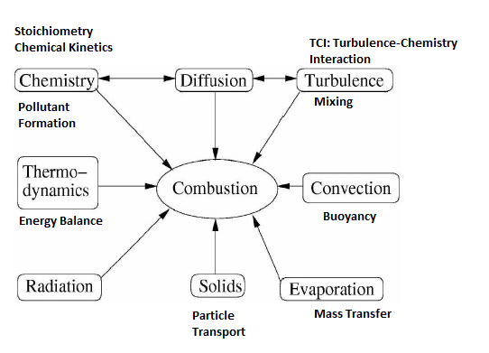
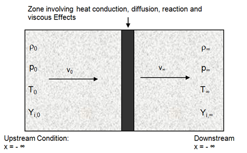
XiFoam, engineFoam, sprayEngineFoam, fireFoam, sprayFoam, reactingFoam are some of the utilities related to combustion in OpenFOAM. Internal combustion engines, industrial furnaces used in metal and cement industries can greatly benefit with increased insight into the combustion system used there.Combustion is one of the most complex phenomena in engineering which requires to deal with turbulent fluid flow, radiative and convective heat transfer, chemical reaction and pollutant formation, mixing and quenching, particle break-up, evaporation and mass transfer. Internal combustion engines, industrial furnaces used in metal and cement industries can greatly benefit with increased insight into the combustion system used there. Combustion in which the flame front travels below the speed of sound is termed turbulent deflagration. Detonation typically refers to flame fronts traveling as speeds higher than sonic speed. Three primary mode of combustion can be nicely summarized in terms of images shown in later paragraphs.
Disclaimer:
This content is not approved or endorsed by OpenCFD Limited, the producer of the OpenFOAM software and owner of the OpenFOAM and OpenCFD trademarks.
Some of the resources from the web are listed below. IPR: the ownership and copyright of these documents lie with the author mentioned in the document.
- This web page from CHALMERS university is a comprehensive list of article, research report and presentations on OpenFOAM
- This is a wiki page which is an excellent attempt to categorize the documents with ease of search.
- fireFoam: pool fire
- sprayFoam (dieselFoam): injector centrally located in a vertical column - lagrangian/sprayFoam/aachenBomb
- Soot model in lagrangian/sprayFoam/aachenBomb
CFD Simulation and Combustion Modeling in OpenFOAM
In addition to standard files and dictionaries required to model any CFD simulation in OpenFOAM, following additional files are required exclusively to model combustion phenomena.Combustion is a chemical reaction. A general reaction is repsetned as a.A + b.B + ... → c.C + d.D + ... where a, b, c, d... are the stoichiometric coefficients of reactants and products. The rate expression for this reaction is Rate ∝ [A]x [B]y where exponents x and y may or may not be equal to the stoichiometric coefficients (a and b) of the reactants. The concentration of species are usually expressed as [kmole/m3] or [mole/cm3] or [mole/L]. The equation can also be expressed as Rate = dR/dt = k [A]x [B]y where k is a proportionality constant called rate constant. The rate of reaction has the unit [kmole/m-s3] or [mole/cm3-s] or [mole/L-s]. The rate of reaction is the molar rate of destruction or creation of an species. The molar value is most consistent since the chemical reaction has to deal with conservation of atoms and this makes use of other units like [kg/m3/s] or [m3/s] impossible to use without associating every value and situation with a known operating temperature and pressure. The term stoichiometric refers to "chemically correct" or theoretical values.
Note that the stochimetric ratio refers to the conditions when both fuel and oxidizer is completely consumed. The ratio can either be in terms of number of moles or mass. Zero order reaction means that the rate of the reaction is proportional to zero power of the concentration of reactants. Thus, Rate = dR/dt = k [R]0. Zero order reactions are relatively uncommon but they occur under special conditions. Some enzyme catalysed reactions and reactions which occur on metal surfaces are a few examples of zero order reactions. The decomposition of gaseous ammonia on a hot platinum surface is a zero order reaction at high pressure.
In 'first order' class of reactions, the rate of the reaction is proportional to the concentration of the reactant R. Rate = dR/dt = k [R]1. Hydrogenation of ethene is an example of first order reaction. All natural and artificial radioactive decay of unstable nuclei take place by first order kinetics.
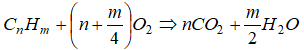
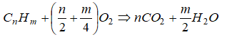
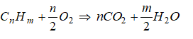
The balanced chemical equation for the complete combustion of a general hydrocarbon fuel CxHy is given by
CxHy + (x + 0.25y)O2 → xCO2 + 0.5y×H2O
Air is a mixture of 20.9% (mole basis) O2 and 79.1% (mole basis) N2. Thus for every mole of oxygen required for combustion, 79.1/20.9 = 3.785 [moles] of nitrogen must be introduced as well. On mass basis, air composition is 23.3% O2 and and 76.7% N2. Thus, the reaction can also be re-written asCxHy + (x + y/4) × (O2 + 3.785N2) → xCO2 + y/2 × H2O + 3.785(x + y/4) × N2
Note:- 1 mole of oxygen requires 1/0.209 = 4.785 [moles] of air and hence 1 mole of fuel requires (x + y/4) moles of oxygen.
- For every mole of fuel burned, 4.785( x + y/4) moles of air are required. Hence, the molar fuel/air ratio for stoichiometric combustion is 1 / [4. 785(x + y/4)] = 0.836/(4x + y).
- The stoichiometric molar air/fuel ratio is 1.196×(4x + y). For methane (CH4), the ratio is 1.196 × (4 × 1 + 4) = 5.98 and for octane (C8H18) the ratio would be 59.8
- For every mole of fuel burned [4. 785(x + y/4) + y/4] moles of combustion products are generated. Gas compositions are generally reported in terms of mole fractions since the mole fraction does not vary with temperature or pressure as does the concentration (moles/unit volume).
- Stoichiometric mass fuel/air ratio = MWFUEL / [(x+y/4) × (32 + 3.785 × 28] = MWFUEL / [(x+y/4) × 137.98]. For octane (C8H18), the ratio is 114 / [(8 + 18/4)× 137.98] = 0.0661 [kg-fuel/kg-air] where 114 [kg/kmole] is molecular weight of the fuel.
- Stoichiometric mass air/fuel ratio = [(x+y/4) × 137.98] / MWFUEL. For octane (C8H18), the ratio is [(8 + 18/4)× 137.98] / 114 = 15.1 [kg-air/kg-fuel]. The value for methane is 17.2 [kg-air/kg-CH4].
CxHyOz + (x + y/4 - z/2) × (O2 + 3.785N2) → xCO2 + y/2 × H2O + 3.785(x + y/4 - z/2) × N2
The equivalence ratio is the ratio of fuel to oxidizer ratio in the unburnt to that of a stoichiometric mixture. That is φ = [F/A]ACTUAL / [F/A]STOICH. Thus: at fuel-rich conditions φ gt; 1) and fuel-lean conditions φ < 1. The stoichiometric ration, λ = 1/φ.
Percent Excess Air: The amount of air in excess of the stoichiometric amount is called excess air. The percent excess air, %EA = 100 (1/φ -1) = 100 (λ -1). Thus: φ = 100 / [%EA + 100].
Enthalpy of combustion or heat of combustion: Ideal amount of energy that can be released by burning a unit amount of fuel. Enthalpy of reaction or heat of reaction: Energy that must be supplied in the form of heat to keep a system at constant temperature and pressure during a reaction.
Global equation for rich combustion: equivalence ratio φ > 1 isCxHyOz + [1/φ].(x + y/4 - z/2) × (O2 + 3.785N2) → [x/φ] CO2 + [y/2φ] × H2O + 3.785/φ.(x + y/4 - z/2) × N2 + (1 - 1/φ) × CxHyOz
Global equation for lean combustion φ ≤ 1 isCxHyOz + [1/φ].(x + y/4 - z/2) × (O2 + 3.785N2) → xCO2 + y/2 × H2O + 3.785/φ.(x + y/4 - z/2) × N2 + (x + y/4 - z/2).(1/φ - 1) × O2
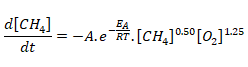
The temperature dependence of the rate of a chemical reaction can be accurately explained by Arrhenius equation. It was first proposed by Dutch chemist, J.H. van’t Hoff but Swedish chemist, Arrhenius provided its physical justification and interpretation. k = A.e-Ea/RT where A is the Arrhenius factor or the frequency factor. It is also called pre-exponential factor. It is a constant specific to a particular reaction. R is gas constant and Ea is activation energy measured in [J/mole].
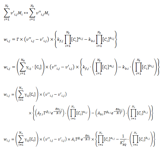
- v'i,j - Stoichimetric coefficient of species ‘i’ appearing as a reactant in reaction 'j'
- v’’i, k - Stoichiometric coefficient of species ‘i’ appearing as a product in reaction j
- Mi - Chemical symbol of species i
- Ns - Number of species in reaction j
- Wi,j - Rate of production or destruction of species i in reaction j
- kf,i - Forward reaction rate constant for reaction i
- kb,i - Backward reaction rate constant for reaction i
- Ci - Concentration of species i
- ai,j - Rate exponent of reactant species i in reaction j
- bi,j - Rate exponent of product species iI in reaction j
- NR - Number of reactions
- Wi,j - Rate of production / destruction of species 'i' in reaction 'j'
- Γ - Net effect of third bodies on the reaction rate
- γij - Third-body efficiency of the species 'i' in reaction 'j'
- KEQj - Equilibrium constant for reaction j
Combustion variables in OpenFOAM
- Flame Wrinkling Parameter Xi [Ξ] refers to the ratio [St/Su] where St is Turbulent Flame (deflagration) Speed and the object Su is Laminar Flame Speed (3 different models: unstrained, equilibrium, transport). The premixed laminar flame speed is proportional to (α R)0.5 where α is a diffusivity and R is a reaction rate. The laminar flame can be artificially thickened, without altering the laminar flame speed, by increasing the diffusivity and decreasing the reaction rate proportionally. The thickened flame can then be feasibly resolved on a coarse mesh while still capturing the correct laminar flame speed. Detonation on the other hand is the result of a supersonic wave initiating a secondary explosion.
- All species fractions are given on mass-basis.
- constant/chemistryProperties - This file under 'constant' folder of the case lists initial chemical time step, ODE solver and solver properties to be used.
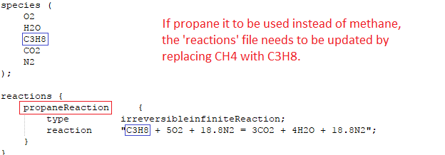
- constant/combustionProperties - Here turbulence chemistry interaction model and model constants are listed. Parameters such as fuel name [e.g. Propane, Methane, IsoOctane], laminar flame speed, equivalence ratio, XiModel, GuldersCoeffs, spark or ignition zone and its location / size / strength / duration, fuel fraction in ignition site ... are specified through this file.
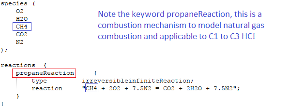
- constant/reactions - The detailed reaction mechanism in native OpenFOAM format (m3, kmole, Joules, K) or CHEMKIN format (mol, cm3, s, K; cal) is specified through this file. The utility chemkinToFoam can be used to convert CHEMKINIII thermodynamics and reaction data files into native OpenFOAM format.
- constant/thermo.compressibleGas - Thermophysical data for the chemical species involved in reactant and product are listed here.
- The initial and boundary conditions, in addition to standard U, p, T files, are specified by additional files such as CH4, CO2, H2O, N2, O2, Ydefault in 0/ directory to store chemical species mass fractions.
- Ydefault specifies initial and boundary conditions for all species other than O2, N2 and fuel such as CH4, C7H16... that appear in reaction mechanism either on the reactants or products side.
- ft is the fuel mass fraction i.e. fuel/(fuel + oxidant [usually air]), fu is unburnt fuel fraction.
- Mean reaction regress variable 'b' - also known as normalized fuel fraction in file 0/b specifies non-dimensional temperature boundary condition at all flow inlets: fresh gas [unburnt mixture] b = 1.0 and burnt gas [burnt mixture] b = 0.0. This is based on assumption that the reaction is effectively instantaneous so the value jumps from 1 to 0 at the flame front.
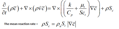
This is analogous to Reaction Progress Variable 'c' in CFX which subdivides the flow field in two different areas, the burnt and the unburnt mixture. In CFX, 'c' is defined as the probability of the reacted state of the premixed fluid. For example, c = 0.8 implies that the fluid (the gas mixture) at a given position is fully reacted during 80% of the time and non-reacted during the remaining 20% of the time. Burnt regions [c ~ 1] are treated as a diffusion flame whereas unburnt regions [c ~ 0] represent cold mixture.
- The object b is defined as b = [TBURNT-GAS - T] / [TBURNT-GAS - TFRESH-GAS], Ξ = Flame Wrinkling Parameter
The code can be expressed as: solve(fvm::ddt(rho, b)+ mvConvection->fvmDiv(phi, b)+ fvm::div(phiSt, b, "div(phiSt,b)") - fvm::Sp(fvc::div(phiSt), b) - fvm::laplacian(turbulence->muEff(), b));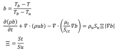
- Tu: Temperature of unburnt gas at the boundaries and internal field is specified by object Tu in the file 0/Tu.
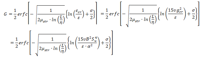
- μstr is the stretch factor coefficient for dissipation pulsation, the default value of 0.26 is suitable for most premixed flames
- L is the turbulent integral length scale
- η is the Kolmogorov micro-scale
- εcr is the turbulence dissipation rate at the critical rate of strain
- gcr is the critical rate of strain: should be set to a very high value (1010) to prevent flame stretching
- B is a constant (typically 0.5)
- α is the thermal diffusivity, also known as molecular heat transfer coefficient. Laminar flame thickness ~ α / Su.
Mole Fraction to Mass Fraction
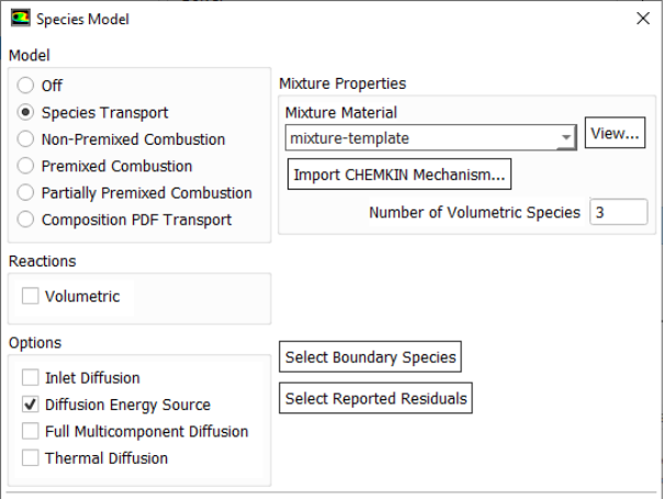
Most of the gaseous fossile fuels are mixture of gases such as 58% CH4 – 20% C2H6 – 12% C3H8 – 10% CO2 for a shale gas. IN ANSYS FLUENT, species transport model allows to use a mixture template to include the composition of the fuel. While specifying the composition of fuel and oxidation stream, one must include the products species such as CO2 and H2O into the mixture even if they are absent in the initial composition.
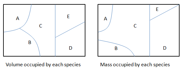
There are 3 different ways to specify the mixture composition: volume fraction, mole fraction and mass fraction of each constituents. It is worth noting that the volume fraction and mole fraction of a consituent in gaseous mixture are always equal. The conversion of volume fraction to mass fraction is explained in table below.
| Species | Volume Fraction | Molecular Weight | Mole Fraction | Mass in Mixture | Mass Fraction |
| i | α | MW | η | mi = MWi × ηi | η = mi / M |
| [ - ] | [ - ] | [g/mole] | [ - ] | [g] | [ - ] |
| A | 0.10 | 30 | 0.10 | 3.00 | 0.0806 |
| B | 0.20 | 16 | 0.20 | 3.20 | 0.0860 |
| C | 0.25 | 28 | 0.25 | 7.00 | 0.1882 |
| D | 0.30 | 58 | 0.30 | 17.4 | 0.4677 |
| E | 0.15 | 44 | 0.15 | 6.60 | 0.1774 |
| Total | 1.00 | - | 1.00 | M = 37.2 | 1.000 |
The composition of natural gas reported in "Advanced modeling of oxy-fuel combustion of natural gas" by Chungen Yin:
| Species | CH4 | C2H6 | C3H8 | C4H10 | C5H12 | CO2 | N2 | O2 |
| %volume | 86.2 | 5.4 | 1.87 | 0.58 | 0.14 | 1.79 | 4.01 | 0.21 |
| Molecular weight: 18.661 [g/mole] | Density at NTP = 0.8325 [kg/m3] | LHV = 44.454 [MJ/kg] | ||||||
| Species | Molecular weight [g/mole] | Formation enthalpy [J/mole] | Molar fraction [%] | Mass fraction [-] |
| C1.122H4.244 | 17.75 | -7.663e+07 | 93.99 | 0.8940 |
| CO2 | 44.0 | -3.935e+08 | 1.79 | 0.0422 |
| N2 | 28.0 | 0 | 4.01 | 0.0602 |
| O2 | 32.0 | 0 | 0.21 | 0.0036 |
| Species | CH4 | C2H6 | C3H8 | C4H10 | C5H12 | Total | Normalized |
| %volume of NG | 86.20% | 5.41% | 1.87% | 0.58% | 0.14% | 94.2% | - |
| %volume of HC | 91.51% | 5.74% | 1.99% | 0.62% | 0.15% | 100% | - |
| Mole fraction | 0.915 | 0.057 | 0.020 | 0.006 | 0.001 | 100% | |
| C-mass [g]: mole fraction × MWC | 10.99 | 1.38 | 0.72 | 0.30 | 0.09 | 13.38 | 1.115 |
| H-mass [g]: mole fraction × MWH | 3.66 | 0.34 | 0.16 | 0.06 | 0.02 | 4.225 | 4.225 |
Flammability Limits and Calorific Values
The lower and upper flammability limits (LFL and UFL respectively) are the limiting fuel concentrations in air that can support flame propagation and lead to an explosion. Fuel concentrations outside those limits are non-flammable. For combustion cases, a value 10% – 50% larger than the stoichiometric mixture fraction can be used for the rich flammability limit of the fuel stream. Similarly, the limiting oxygen concentration (LOC) is the minimum O2 concentration in a mixture of fuel, air, and an inert gas that will propagate flame. As the concentration of inert gas such as N2 and He is increased, the LFL increase and UFL decrease and may reach to a point where both coincide. The lower flammability limit (LFL) for mixtures of gaseous fuels is adequately given by the Le Chatelier rule: LFLMIX = 1 / Σ(ηi/LFLi).
When a combustible gas [hydrocarbon, hydrogen, refrigerants...] leaks into a confined space where an ignition source [e.g. hot surface such as electric plugs] could be present, there is a possibility of fire and/or explosion taking place. The UFL and LFL for the refrigerant R32 are 14.4% and 29.3% by volume, respectively [Safety data sheet by National Refrigerants Inc]. For confined spaces, Flammability Volume, FV is defined as the volume of leaked gas that is between the UFL and LFL. This helps estimate the probability of a fire as well as magnitude of an event. Normalized Flammability Volume (NFV) is ratio of FV and volume to the confined space which represents the probability of a fire/explosion occurring assuming the ignition sources are randomly distributed in the entire room.
The gross or higher calorific value (HCV) usually expressed as [MJ/kg] or [MJ/m3] is defined as the quantity of heat produced by the complete combustion, at a constant pressure equal to 101325 [Pa] of a unit volume or mass of gas, the constituents of the combustible mixture being taken at reference conditions and the products of combustion being brought back to the same conditions and where the water produced by combustion is assumed to be condensed. The main combustion related property as it is used in the natural gas industry, is the Wobbe index W = HCV / d0.5 where d = relative density (dimensionless).
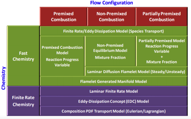
Modeling Species Transport and Finite-Rate Chemistry
Excerpts from FLUENT user guide: "mixing and transport of chemical species by solving conservation equations describing convection, diffusion, and reaction sources for each component specie. Multiple simultaneous chemical reactions can be modeled, with reactions occurring in the bulk phase (volumetric reactions) and/or on wall or particle surfaces, and in the porous region. In many cases, you will not need to modify any physical properties because the solver gets species properties, reactions... from the materials database when you choose the mixture material. Some properties, however, may not be defined in the database. You will be warned when you choose your material if any required properties need to be set and you can then assign appropriate values for these properties."Turbulent reacting flame can be modeled using the mixture fraction approach (for non-premixed systems), the reaction progress variable approach (for premixed systems), the partially premixed approach or the composition PDF Transport approach. The calculation will be performed assuming that all properties except density and specific heat are constant. The constant transport properties (viscosity, thermal conductivity and mass diffusivity coefficients) is reasonably accurate when the flow is fully turbulent. The molecular transport properties will play a minor role compared to turbulent transport.
Hydrocarbon fuel combustion mechanisms share four types of elementary reactions:- Ignition (initiation)
- Propagation - chain carrying
- Propagation - chain branching
- Termination (extinction)
Reference Data
Rate parameters for quasi-global reaction mechanisms giving best agreement between experimental and computed flammability limits (Flagan and Seinfeld, 1988; Westbrook and Dryer, 1981) (units: m, s, mol, K).Single-step Mechanism: This model does not include intermediate hydrocarbon species or carbon monoxide. Excerpt from Simplified Reaction Mechanisms for the Oxidation of Hydrocarbon Fuels in Flames by CHARLES K. WESTBROOK and FREDERICK L. DRYER - "A global reaction is often a convenient way of approximating the effects of the many elementary reactions which actually occur. Its rate must therefore represent an appropriate average of all of the individual reaction rates involved. The rate expression of the single reaction is usually expressed as ROV = A Tn e-Ea/RT [Fuel]a [O2]b where [...] denotes concentration of the species in units such as [kmole/m3] or [mole/cm3] or [mole/L]. Here n is called temperature exponent, a and b are concentration exponents. The simplest overall reaction representing the oxidation of a conventional hydrocarbon fuel is expressed as [Fuel] + n1O2 = n2CO2 + n3H2O.
The most common assumption in the combustion literature for the concentration exponents is that the rate expression is first order in both fuel and oxidizer i.e. a = b = 1. This is true mostly near stoichiometric fuel-air ratio. The computed flame speeds particularly for rich mixtures deviate significantly with this approximation. Hence, this rate expression should not be used in models for any combustion problems in which the fuel-air equivalence ratio varies with time or position.
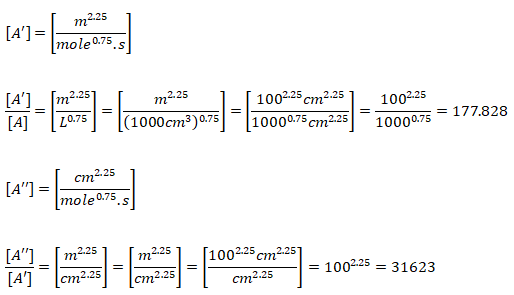
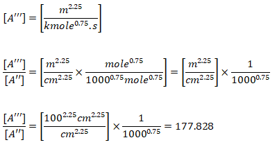
Note that the original reaction rate parameters tabulated by Westbook and Dryer [WD] use units [cm-sec-mole-kcal-Kelvin]. Hence, the rate of reaction will be in [mole/cm3-s]. If units used are [m-sec-kmole-kJ-Kelvin], the value of A will need to be divided by 10000.75 = 177.828 and the rate of reaction will have the units [kmole/m3-s]. Note that kmole is also expressed as kgmole in some texts and programs such as ANSYS FLUENT. 1 [mole/cm3/s] = 10-3[kmol]/10-6[m3]/s and hence 1 [mole/cm3/s] = 1000 [kmole/m3/s]. Since the exponent of mole fractions of reactants sum to 1.75, the conversion factor 1000 needs to be scaled by factor 10001.75 - 1.00 = 0.75. Also note that the pre-exponential factor has the same unit as reaction rate coefficient (consistent units with concentration and rate of reaction). Also, Ea [J/kgmole] = 1000 * Ea [J/mole].
 , rate of reaction are in [kmole/m3-s] , rate of reaction are in [kmole/m3-s] | ||||||
| Fuel | A [ - ] | Ea/R [K] | a [ - ] | b [ - ] | Ea [J/mole] | Ea [kcal/mole] |
| CH4 | 1.300×10⁹ | 24400 | -0.30* | 1.30 | 202862 | 48462 |
| C2H2 | 3.665×10¹⁰ | 15000 | 0.50 | 1.25 | 124710 | 29792 |
| C2H4 | 1.125×10¹⁰ | 15000 | 0.10 | 1.65 | 124710 | 29792 |
| C2H6 | 6.186×10⁹ | 15000 | 0.10 | 1.65 | 124710 | 29792 |
| C3H8 | 4.836×10⁹ | 15000 | 0.10 | 1.65 | 124710 | 29792 |
| CH3OH | 1.800×10¹⁰ | 15000 | 0.25 | 1.50 | 124710 | 29792 |
| C2H5OH | 8.440×10⁹ | 15000 | 0.15 | 1.60 | 124710 | 29792 |
| C6H6 | 1.120×10⁹ | 15000 | -0.10 | 1.85 | 124710 | 29792 |
| C8H18 | 2.590×10⁹ | 15000 | -0.10 | 1.85 | 124710 | 29792 |
Some papers such as "Simulation of turbulent piloted methane non-premixed flame based on combination of finite-rate/eddy-dissipation model" in ISSN 1392 - 1207. MECHANIKA. 2013 Volume 19(6): 657-664 reports following constants for WD1 mechanims.
| WD1 Reaction: CGS units: concentration is in [mole/cm3/s] | A [ - ] | Ea [J/mole] | a | b | β |
| (i) CH4 + 2O2 → CO2 + 2H2O | 1.00e+12 | 1.0e+08 | 0.50 | 1.25 | 0 |
Two-step Mechanism: During combustion, the oxidation of hydrocarbons occurs quickly. The oxidation of CO to CO2 is slower. Combining all the reactions that comprise CO oxidation does not accurately describe what actually happens soon after ignition. This model is adequate if one is interested in processes that occur later in combustion.
 rate of reaction are in [kmole/m3-s] rate of reaction are in [kmole/m3-s] | ||||
| Fuel | A [ - ] | Ea/R [K] | a | b |
| CH4 | 1.575E+07 | 24400 | 0.70 | 0.80 |
| C2H2 | 4.386E+10 | 15000 | 0.50 | 1.25 |
| C2H4 | 1.350E+10 | 15000 | 0.10 | 1.65 |
| C2H6 | 7.310E+09 | 15000 | 0.10 | 1.65 |
| C3H8 | 5.623E+09 | 15000 | 0.10 | 1.65 |
| CH3OH | 2.081E+10 | 15000 | 0.25 | 1.50 |
| C2H5OH | 1.012E+10 | 15000 | 0.15 | 1.60 |
| C6H6 | 1.350E+10 | 15000 | -0.10 | 1.85 |
Excerpt from Simplified Reaction Mechanisms for the Oxidation of Hydrocarbon Fuels in Flames by CHARLES K. WESTBROOK and FREDERICK L. DRYER - "The single-step mechanism predicts flame speeds reliably over considerable ranges of conditions, but it has several flaws which can be important in certain applications. By assuming that the reaction products are CO2 and H2O, the total heat of reaction is overpredicted. At adiabatic flame temperatures typical of hydrocarbon fuels (~ 2000 K) substantial amounts of CO and H2 exist in equilibrium in the combustion products with CO2 and H2O. The same is true to a lesser extent with other species, including some of the important free radical species such as H, O and OH. This equilibrium lowers the total heat of reaction and the adiabatic flame temperature below the values predicted by single step mechanism."
Two-step mechanism for methane-air: (i)CH4 + 1.5O2 → CO + 2H2O, (ii)CO + 0.5O2 ↔ CO2
Four-step mechanism for methane-air (Jones-Lindstedt Mechanism): (i)CH4 + 0.5O2 → CO + H2O, (ii)CH4 + H2O → CO + 3H2,(iii)CO + H2O ↔ CO2 + H2 and (iv)H2 + 0.5O2 ↔ H2O
The frequency factor, activation energy and rate exponents for 4-step mechanism for methane as per Jones-Lindstedt (JL) are tabulated below.| JL4 Reaction: CGS units: concentration is in [mole/cm3/s] | A [ - ] | Ea [kcal/mole] | a | b | β |
| (i) CH4 + 0.5O2 → CO + H2O | 7.82e+13 | 30 | 0.50 | 1.25 | 0 |
| (ii) CH4 + H2O → CO + 3H2 | 3.00e+11 | 30 | 1.00 | 1.00 | 0 |
| (iii) CO + H2O ↔ CO2 + H2 | 2.75e+12 | 40 | 1.00 | 1.00 | -1 |
| (iv)H2 + 0.5O2 ↔ H2O | 1.21e+18 | 20 | 0.25 | 1.50 | 0 |
For reactions (i) and (iv), the unit of A is [cm2.25/mole0.75.s] and for reactions (ii) and (iii), the unit of A is [cm3/mole.s].
| JL4 Reaction:[cal, mole, L, s] units: concentration is in [mole/L/s] | A [ - ] | Ea [kcal/mole] | a | b | β |
| (i) CH4 + 0.5O2 → CO + H2O | 4.40e+11 | 30 | 0.50 | 1.25 | 0 |
| (ii) CH4 + H2O → CO + 3H2 | 3.00e+08 | 30 | 1.00 | 1.00 | 0 |
| (iii) CO + H2O ↔ CO2 + H2 | 2.75e+09 | 40 | 1.00 | 1.00 | -1 |
| (iv) H2 + 0.5O2 ↔ H2O | 6.80e+15 | 20 | 0.25 | 1.50 | 0 |
Note that in reactions (ii) and (iii), the sum of exponents a + b = 1 and hence conversion from [cal, mole, L, s] to [cal, mole, cm, s] unit required a multiplication of 1000. Note 1 [L] = 1000 [cm3]. In the other two cases, the sum of exponents a + b = 1.75 and hence the conversion factor is 10000.75 as explained earlier. For reactions (i) and (iv), the unit of A is [L0.75/mole0.75.s] and for reactions (ii) and (iii), the unit of A is [L/mole.s].
| WD3 Reaction:[cal, mole, L, s] units: concentration is in [mole/L/s] | A [ - ] | Ea [kcal/mole] | a | b | β |
| CH4 + 1.5O2 → CO + 2H2O | 5.00e+11 | 47.8 | 0.70 | 0.80 | 0 |
| CO + 0.5H2O → CO2 | 2.24e+12 | 40.7 | 1.00 | 1.00 | 0 |
| CO2O ↔ CO + 0.5O2 | 5.00e+08 | 40.7 | 1.00 | - | 0 |
![pre-Exponential Factor in [L/mole.s]](Images/preExpFactor_L_mole_s.png)
Quasi-global Mechanism: Additional reactions has been worked out in quasi-global mechanisms to improve agreement between models and test data. For example, the oxidation of fuel to form an intermediate hydrocarbon and H2 is modeled by a single reaction. Then, detailed mechanisms are used to describe the oxidation of ethene and H2. Other quasi-global models start by representing the oxidation of fuel to form CO and H2 with a single reaction. Then, detailed mechanisms are used to describe the oxidation of CO and H2.
 rate of reaction are in [kmole/m3-s] rate of reaction are in [kmole/m3-s] | ||||
| Fuel | A [ - ] | Ea/R [K] | a | b |
| CH4 | 2.249E+07 | 24400 | -0.30 | 1.30 |
| C2H2 | 6.748E+10 | 15000 | 0.50 | 1.25 |
| C2H4 | 2.418E+10 | 15000 | 0.10 | 1.65 |
| C2H6 | 1.125E+10 | 15000 | 0.30 | 1.30 |
| C3H8 | 8.435E+09 | 15000 | 0.10 | 1.65 |
| CH3OH | 4.105E+10 | 15000 | 0.25 | 1.50 |
| C2H5OH | 2.024E+10 | 15000 | 0.15 | 1.60 |
| C6H6 | 2.418E+09 | 15000 | -0.10 | 1.85 |
| Decription | 1-step global reaction | 2-step reaction (WD) | 4-step reaction (JL) | Full dissociation |
| Air-CH4 | 2326 | 2256 | 2245 | 2223 |
| Species | CO2, H2O | CO, CO2, H2O | CO, CO2, H2, H2O | No. of species ≥ 100 |
CHEMKIN to OpenFOAM Format: Note that the chemkinToFoam utility updates the data for Specific Heat Capacity only and the transport data for temperature coefficients of viscosity needs to be updated manually.

H/RT = a1 + a2 * T/2 + a3 * T2 / 3 + a4 * T3 / 4 + a5 * T4 / 5 + a6 / T
S/R = a1 ln(T) + a2 * T + a3 * T2 / 2 + a4 * T3 / 3 + a5 * T4 / 4 + a7
Here a1, a2, a3, a4, a5, a6 and a7 are constant coefficients.
- Tlow, Thigh and Tcommon defines Lower, Upper and Common temperature respectively.
- The first 7 numbers starting on the second line of each species entry are the seven coefficients (a1, a2 ... a7 respectively) for the high-temperature range. a7 is the entropy offset.
- The next seven numbers are the coefficients (a1, a2 ... a7 respectively) for the low-temperature range.
- Sub-dictionary 'transport' contains Sutherland coefficient.
- H is defined as H(T) = ΔHf(298) + [H(T) - H(298 K)]. Thus, in general H(T) is not equal to ΔHf(T) and hence the data for the reference elements is required to calculate ΔHf(T).
Reacting Flows Models in ANSYS FLUENT
Note that there is not unit mentioned for Pre-Exponential Factor even though there is a unit for Activation Energy {J/kgmole]. This does not mean that the Pre-Exponential Factor is dimensionless, it only meant that the value should be used consistent with the fuel concentration units say [mole/L] or [kg/m3]....
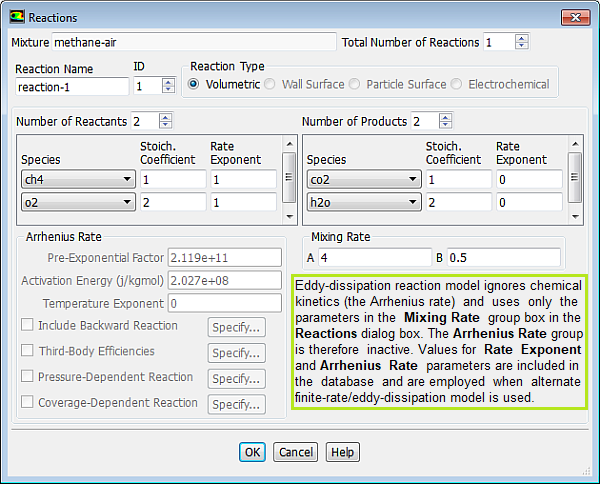
Mixing rate 'A' is Magnussen constant for reactants (default 4.0) and B is Magnussen constant for products (default 0.5). The model Finite Rate / Eddy Dissipation Moel (FR-EDM) always requires some product to be present for reactions to proceed. If this is not desirable, initial mass fractions of product say 1.0E-05 can be patched or specified during intialization stage. 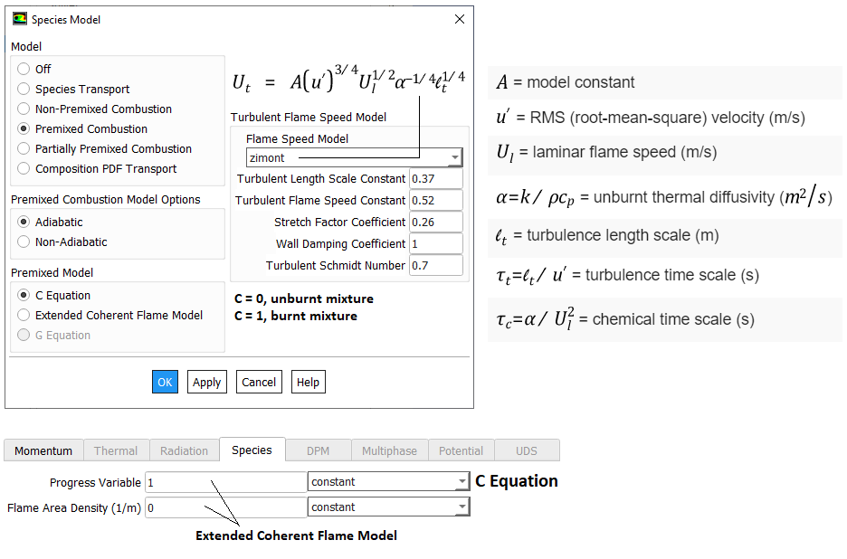
Combustion Solvers in OpenFOAM
The solvers related to combustion and chemical reaction are reactingFoam, XiFoam, rhoReactingFoam, PDRFoam (Porosity/Distributed Resistance solver such as for flame propagation over obstacles in HRSG - its development was funded by Shell), sprayFoam (earlier known as dieselFoam), reactingMultiphaseEulerFoam, reactingTwoPhaseEulerFoam. sprayFoma models flows involving compressible reacting flow with Lagrangian evaporating particles (such as diesel engines) in a three-dimensional domain.
Combustion Mechanism
Combustion depends directly on mixing of the fuel and oxidizer and chemistry involved in reaction between the two. Thus, the relative speed of chemical reaction to mixing is important to characterize the phenomena. Damköhler Number (Da) is an important dimensionless number which represents the ratio of the characteristic turbulent mixing time to the characteristic chemical reaction time i.e. Da = Mixing Time Scale / Chemical Time Scale.- Fast Reactions: reaction rate is limited by turbulent mixing. Here, Da >> 1, chemical reaction rates are fast: mixing limited progress of combustion. Eddy Dissipation Model (EDM) are used in some of the commercial programs in this case. In other words, the eddy-dissipation model computes the rate of reaction under the assumption that chemical kinetics are fast compared to the rate at which reactants are mixed by turbulent fluctuations (eddies). In an eddy dissipation model:
- mixed-is-burned approximation
- instantaneous burn upon mixing
- combustion is mixing limited
- complex chemical kinetics rates are ignored
- Slow Reactions: reaction rate is limited by chemical kinetics. Here Da << 1, chemical reaction rates are slow: chemistry limits progress of combustion. Finite Rate Chemistry Model (FRC) is appropriate for these cases.
- Conservation of mass and species has to be enforced in all combustion models.
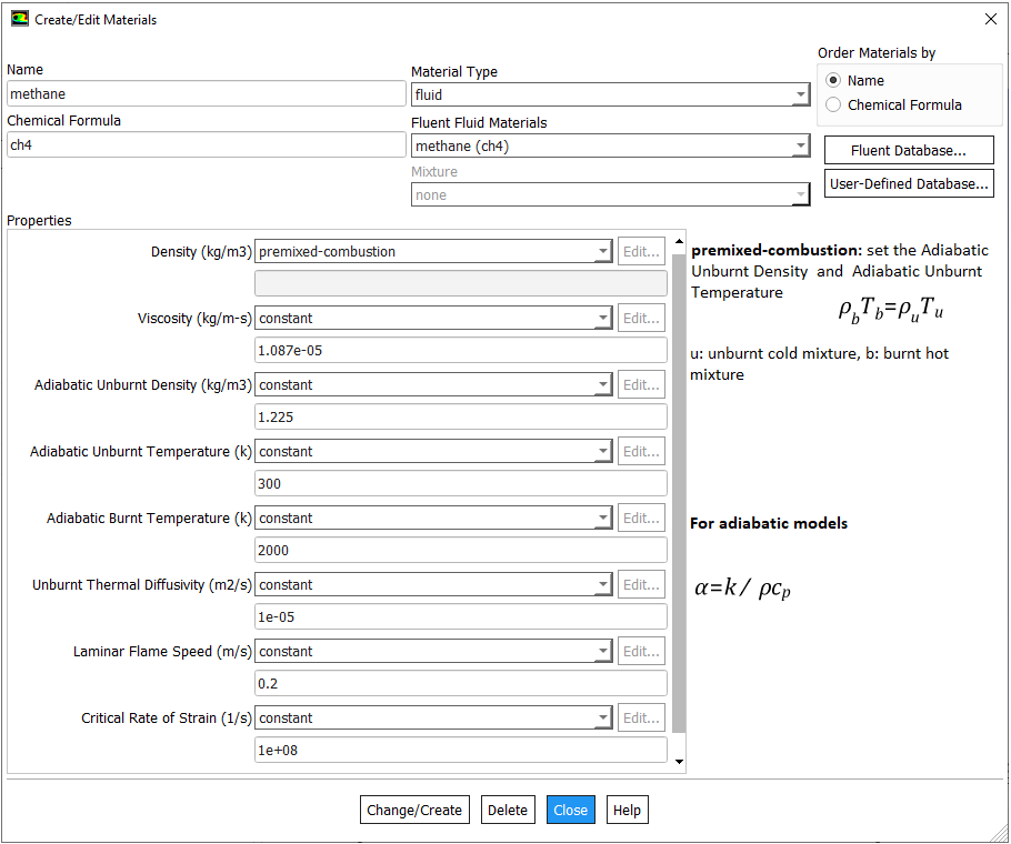
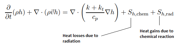
Combustion of homogeneous fuel-air mixture: in ANSYS FLUENT, PDF Mixture Fraction model represents the transport of species by adding two equations, one of the average mixing fraction and another for the variance of the average mixture fraction. In furnaces and in most of the industrial combustions, heat transfer occurs more than 80 % by radiation. To represent this phenomenon and indispensable for determining the correct flame temperature, a radiation model is required. In FLUENT, the Discrete Ordinate Model (DOM) is the most robust model which covers the widest range of optical thickness. Additionally, it is important to take into account the influence of the flue gases (participating media) in radiation, which are mainly triatomic gases water vapor and CO2. The emissivity of these gases in FLUENT is calculated with the weighted sum of gray gases model (WSGGM) - set in material definition for variable "Radiation Absorption Coeff". The material definition also requires "critical flame strain rate" as input. The value of 3000 [1/s] can be set which is the lower bound for the typical range of near-stoichiometric methane flames. Typical values for CH4 lean premixed combustion range from 3000 to 8000 [s−1].
fireFoam -- simulation of transport of heat and smoke in fire incidents. Excerpts from <<Verification, validation and evaluation of FireFOAM as a tool for performance design>> - "There are mainly two versions of FireFOAM code. One is released as a solver for transient fire and diffusion flame simulation by Open CFD (an official release). The other is an extended version of the official release, and it is maintained by FM Global consisting of modified libraries, solvers and cases for fire research."
Fires are essentially diffusion flames where fuel and air are mixing while burning as the fire propagates and increase in size and intensity. Thus, fireFoam is a turbulent diffusion combustion model. The OpenFOAM version includes fireFoam solver with "LES turbulence model" and has capability of simulating Lagrangian sprays such water sprinkler sprays for fire suppression. E.g. combustion>>fireFoam>>les>>flameSpreadWaterSuppressionPanel. As per the source code fireFoam.C, fireFoam is a "Transient solver for fires and turbulent diffusion flames with reacting particle clouds, surface film and pyrolysis modelling." Finite volume discrete ordinates model (fvDOM) is to solve radiation heat transfer equation.
The desired objective to simulate fire phenomena is to get insight into fire detection, heat transfer and temperature rise of structures and smoke expansion / filling rates. Due to sheer scale and hazard of fire, actual testing and measurements are not only expensive sometime impossible.
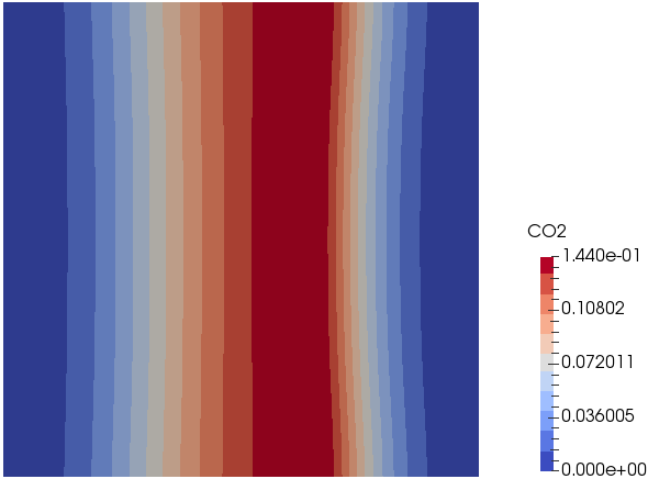
This simple tutorial case is a 2D domain where methane is supplied through a small opening at the bottom face. The combustion model used is infinitelyFastChemistry and no pyrolysisZone is active.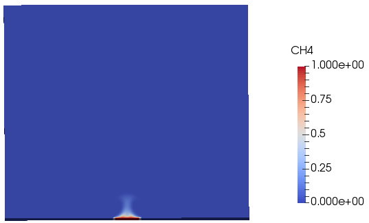
The variation of concentration of methane and CO2 with time and space are shown in the following video.
A tutorial case with 3D version of such phenomena is modelled using a cubical box as shown below.
 Backdraft is one of the hazardous phenomena occurring during fire in a closed space such as buildings. The phenomenon arises from a
sudden entry of fresh air via a gravity current, into a closed space where a fire has been burning. This space has accumulated an excess amount of fuel vapour (as all oxygen gets comsumed fast) and with an ignition source results in a deflagration (turbulence flames).
Backdraft is one of the hazardous phenomena occurring during fire in a closed space such as buildings. The phenomenon arises from a
sudden entry of fresh air via a gravity current, into a closed space where a fire has been burning. This space has accumulated an excess amount of fuel vapour (as all oxygen gets comsumed fast) and with an ignition source results in a deflagration (turbulence flames).
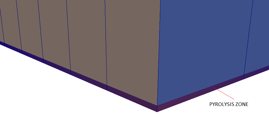
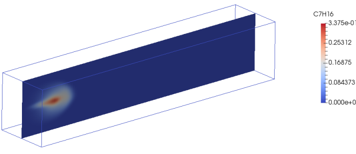
sprayFoam: Diesel Spray Combustion with Lagrangian method - lagrangian/sprayFoam/aachenBomb
The link of PDF tutorial is given at the beginning of this page. Two sample contour plots for concentration of heptane at two time steps are shown below. Key features of combustion in fuel spray injections are:- Strong interaction between turbulence and chemistry.
- Fine droplets size << mesh size keeping in mind limitations on computational resource.
- Lagrangian modeling of spray droplets or parcels eliminating the need to fully resolve the spray region near injector.
- Necessity to model collision, evaporation and break-up of atomized fuel parcels.

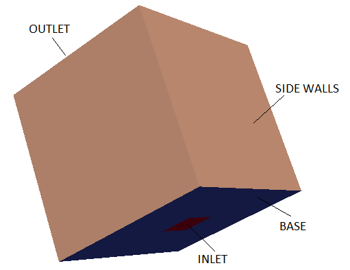
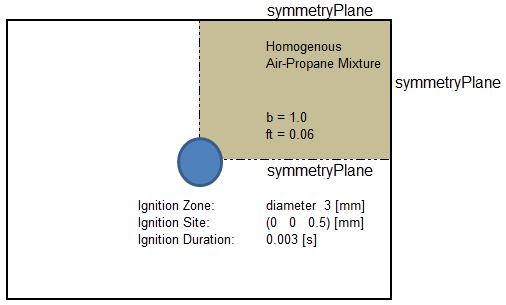
XiFoam - premixed and partially pre-mixed turbulent combustion
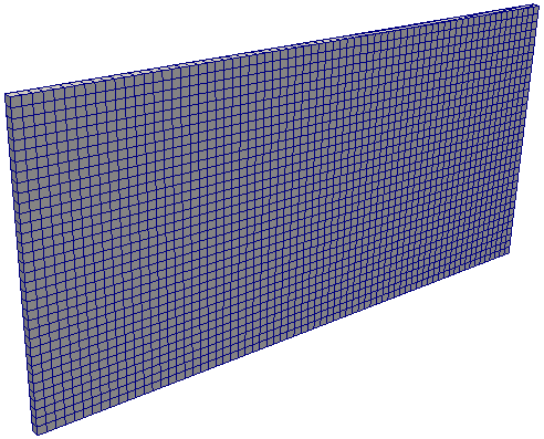
XiFoam: Homogeneous Combustion of Propane - the computational domain is shown by following images.
Temperature at various time [in seconds] are shown below.
Temperature: t = 0.005![XiFoam Temperature t = 0.005 [s]](OpenFOAM/XiFoam_T_005s.png)
![XiFoam Temperature t = 0.010 [s]](OpenFOAM/XiFoam_T_010s.png)
![XiFoam Temperature t = 0.015 [s]](OpenFOAM/XiFoam_T_015s.png)
![XiFoam Temperature t = 0.020 [s]](OpenFOAM/XiFoam_T_020s.png)
reactingFoam
- This is a transient, incompressible solver based on PIMPLE algorithm for non-premixed turbulent combustion of gaseous hydrocarbons.
- The turbulence-chemistry interaction models available for this solver are [a] infinitelyFastChemistry - a single step combustion reaction and [b] diffusion based combustion model - also based on single step combustion reaction. [c] PaSR: Partially Stirred Reactor - a finite rate chemistry model based on both turbulence and chemistry time scales.
- The compressible version is rhoReactingFoam
- 0/Ydefault file is used in case many type of species share a common set of boundary conditions i.e. a default set which is useful in case there are many species involved.
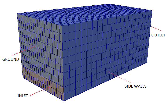
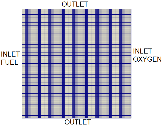
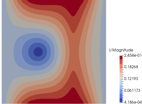
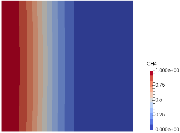
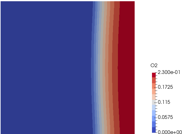
Mixing and Combustion of Methane and Oxygen - the computational domain is shown by following images.
Velocity Magnitude: t = 0.5 [s]
Mass Fraction of Methane: t = 0.5 [s]
Mass Fraction of Oxygen: t = 0.5 [s]
Temperature: t = 0.5 [s]
combustionProperties file with comments
/* Comments based on A Brief tutorial for XiFoam in OpenFOAM 1.7.x by Ehsan
Yasari and Simulating the combustion of gaseous fuels 6th OpenFOAM Workshop
Training Session by Dominik Christ and files in tutorial folders             */

// Gulders, GuldersEGR, constant, SCOPE (PDRFoam);
laminarFlameSpeedCorrelation Gulders;

//----------------------------------------------------------------------------
/* Partially Stirred Reactor [PaSR] model -
   coalChemistryFoam, sprayFoam, simpleReactingParcelFoam                   */
/*
combustionModel  PaSR<psiChemistryCombustion>;
active  true;    //False
PaSRCoeffs  {
    Cmix                1.0;
    turbulentReaction   on;     // sprayFoam: set to 'yes';
	useReactionRate     true;   // simpleReactingParcelFoam
}
*/
//----------------------------------------------------------------------------
// must be specified, if Gulders/GuldersEGR is selected above
fuel                    Propane;
//fuelFile              "fuels/propane.dat";  //PDRFoam

//Laminar Flame Speed - if laminarFlameSpeedCorrelation = constant
Su                      Su [0 1 -1 0 0 0 0] 0.434;

//model  to calculate laminar flame speed: unstrained, equilibrium, transport
SuModel                 unstrained;

// The ratio [fuel-to-oxidizer ratio] / [stoichiometric fuel-to-oxidizer ratio]
equivalenceRatio equivalenceRatio [0 0 0 0 0 0 0] 1;

// The strain rate at extinction which obtained from the Markstein length by
// extrapolating to Su --> 0
sigmaExt                sigmaExt [0 0 -1 0 0 0 0] 100000;

/*Methods  to calculate the Xi parameters: [1] fixed (Xi = constant),
  [2]algebraic: Xi == scalar(1)+
     (scalar(1)+(2*XiShapeCoef)*(scalar(0.5)-b))*XiCoef*sqrt(up/(Su+SuMin))*Reta;
  [3]transport: solve a transport equation for Xi                            */
XiModel                 transport;

//Coefficients used in algebraic model for Xi
//Xi = 1 + [1 + 2 * XiShapeCoef *(0.5 - b)] * XiCoef * sqrt[u' / (Su + Su_Min)] * R_eta
//R_eta = u' / sqrt(epsilon * tau_eta)
//tau_eta = sqrt(mu_unburnt / epsilon / rho_unburnt)
XiCoef                  XiCoef [0 0 0 0 0 0 0] 0.62;
XiShapeCoef             XiShapeCoef [0 0 0 0 0 0 0] 1;

//calculation of velocity fluctuation: u(t) = u_mean + u'
//u' = uPrimeCoef * sqrt(2*k/3), k = TKE (Turbulent Kinetic Energy)
uPrimeCoef              uPrimeCoef [0 0 0 0 0 0 0] 1;

//Coefficients for calculation of laminar flame speed according to the Gulders
//formulation for specific fuel.
GuldersCoeffs {
  Methane     {
    W               0.422;
    eta             0.15;
    xi              5.18;
    alpha           2;
    beta            -0.5;
    f               2.3;
  }
  Propane     {
    W               0.446;
    eta             0.12;
    xi              4.95;
    alpha           1.77;
    beta            -0.2;
    f               2.3;
  }
  IsoOctane    {
    W               0.4658;
    eta             -0.326;
    xi              4.48;
    alpha           1.56;
    beta            -0.22;
    f               2.3;
  }
}

RaviPetersenCoeffs  {
  HydrogenInAir      {
    TRef            320;
    pPoints         ( 1.0e05 5.0e05 1.0e06 2.0e06 3.0e06 );
    EqRPoints       (0.5 2.0 5.0);
    alpha           ( ( (-0.03   -2.347   9.984  -6.734  1.361)
                      ( 1.61   -9.708  19.026 -11.117  2.098)
                      ( 2.329  -12.287 21.317 -11.973  2.207)
                      ( 2.593  -12.813 20.815 -11.471  2.095)
                      ( 2.728  -13.164 20.794 -11.418  2.086) )
                      ( ( 3.558   0.162  -0.247   0.0253 0    )
                      ( 4.818  -0.872  -0.053   0.0138 0    )
                      ( 3.789  -0.312  -0.208   0.028  0    )
                      ( 4.925  -1.841   0.211  -0.0059 0    )
                      ( 4.505  -1.906   0.259  -0.0105 0    ) ) );
    beta            ( ( ( 5.07   -6.42    3.87  -0.767)
                      ( 5.52   -6.73    3.88  -0.728)
                      ( 5.76   -6.92    3.92  -0.715)
                      ( 6.02   -7.44    4.37  -0.825)
                      ( 7.84  -11.55    7.14  -1.399) )
                      ( ( 1.405   0.053   0.022  0    )
                      ( 1.091   0.317    0     0    )
                      ( 1.64   -0.03    0.07   0    )
                      ( 0.84    0.56    0      0    )
                      ( 0.81    0.64    0      0    ) ) );
  }
}
// yes or no
ignite          yes;
ignitionSites  (
  {
    location        (0.0 0.0 0.0005);
    diameter        0.003;
    start           0.0;
    duration        0.003;
    strength        2.0;
  }
);

ignitionSphereFraction                1;
ignitionThickness ignitionThickness   [0 1 0 0 0 0 0] 0.001;
ignitionCircleFraction                0.5;
ignitionKernelArea ignitionKernelArea [0 2 0 0 0 0 0] 0.001;
thermophysicalProperties file with comments
thermoType  {
  type            heheuPsiThermo;
  mixture         homogeneousMixture;
  //singleStepReactingMixture; reactingMixture [sprayFoam]; inhomogeneousMixture;
  transport       sutherland;
  thermo          janaf;
  equationOfState perfectGas;
  specie          specie;
  energy          absoluteEnthalpy;     //sensibleEnthalpy;
}

stoichiometricAirFuelMassRatio stoichiometricAirFuelMassRatio [0 0 0 0 0 0 0] 15.675;

//homogeneousMixture: reactants, inhomogeneousMixture: fuel, oxidant
reactants {
  specie   {                            //keyword
    nMoles          24.8095;
    molWeight       29.4649;
  }
  thermodynamics     {
    Tlow            200;              //Lower, Upper and Common temperatures
    Thigh           5000;
    Tcommon         1000;
   // Cp / R = a1 + a2 * T + a3 * T^2 + a4 * T^4 + a5 * T^5, a6:enthalpy offset,a7:entropy offset
    highCpCoeffs    (3.28069 0.00195035 -6.53483e-07  1.0024e-10 -5.64653e-15 -1609.55 4.41496);
    lowCpCoeffs     (3.47696 0.00036750  1.84866e-06 -9.8993e-10 -3.10214e-14 -1570.81 3.76075);
  }
  transport  {                  //Sutherland coefficient, mu = As /[1+Ts/T] * [Ts]^0.5
    As              1.67212e-06;
    Ts              170.672;
  }
}

// inhomogeneousMixture only
/*
oxidant   {
  specie     {
  nMoles          1;
  molWeight       28.8504;
  }
  thermodynamics    {
  Tlow            200;
  Thigh           6000;
  Tcommon         1000;
  highCpCoeffs    ( 3.10131 0.00124137 -4.18816e-07 6.64158e-11 -3.91274e-15 -985.266 5.35597 );
  lowCpCoeffs     ( 3.58378 -0.000727005 1.67057e-06 -1.09203e-10 -4.31765e-13 -1050.53 3.11239 );
  }
  transport    {
    As              1.67212e-06;
    Ts              170.672;
  }
}
*/ inhomogeneousMixture only

//homogeneousMixture: products, inhomogeneousMixture: burntProducts,
products  {
  specie     {
    nMoles          1;
    molWeight       28.3233;
  }
  thermodynamics     {
    Tlow            200;
    Thigh           5000;
    Tcommon         1000;
    highCpCoeffs    (3.1060 0.00179682 -5.94382e-07 9.04998e-11 -5.08033e-15 -11003.7 5.11872);
    lowCpCoeffs     (3.4961 0.00065036 -2.08029e-07 1.22910e-09 -7.73697e-13 -11080.3 3.18978);
  }
  transport     {
    As              1.67212e-06;
    Ts              170.672;
  }
}

// singleStepReactingMixture; reactingMixture;
/*
inertSpecie              N2;
fuel                     CH4;
chemistryReader          foamChemistryReader;
foamChemistryFile        "$FOAM_CASE/constant/reactions";
foamChemistryThermoFile  "$FOAM_CASE/constant/thermo.compressibleGas";       */

//sprayFoam
//CHEMKINTransportFile     "$FOAM_CASE/chemkin/transportProperties";

//sprayFoam
/*
liquids  {
  C7H16     {
   defaultCoeffs   yes;
  }
}
solids  {
  // none
}
*/
Combustion Simulation in IC Engines
coldEngineFoam, engineFoam, moveEngineMesh, sprayEngineFoam, engineCompRatio, engineSwirl are some of the utilities available in OpenFOAM. moveEngineMesh only move the mesh and intended to ensure the mesh motions are working properly and to determine if the mesh quality will be acceptable during the compression/expansion strokes. coldEngineFoam is engineFoam without combustion. In the solver engineFoam, "no special pre-processing for movement of pistons is required because mesh motion is integrated in the solver where at every time step mesh nodes are moved and mesh topology eventually changed when needed. Thus, a mesh is used for a certain crank angle interval (CA) only. However, no new layer of mesh is generated with setting "engineMesh layered;" in engineGeometry dictionary. The mesh is compressed and expanded as the piston moves towards TDC and BDC respectively.
The main consideration of an engine mesh is to have separate patches for cylinder head, liner and piston and the appropriate values in the dictionary engineGeometry. engineMesh will still work with additional patches other than the three mentioned above but only the liner and piston patches will move, everything else will stay stationary. Other patches can be moved using utility fvMotionSolverEngineMesh.
engineCompRatio Calculate the geometric compression ratio. As described in the source code, "Note that if you have valves and/or extra volumes it will not work, since it calculates the volume at BDC and TCD".
Geometry associated with tutorial kivaTest is shown below. 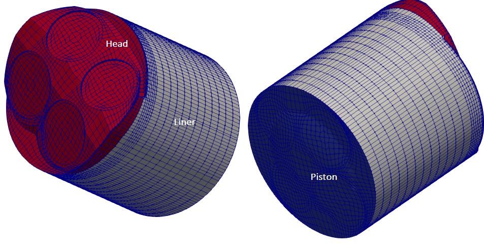
The animation of temperature profile is embedded below. This is an example of spark ignition and this case cannot be used to simulation combustion of diesel injection.
Excerpt from engineFoam.C:
Solver for internal combustion engines. Combusting RANS code using the b-Xi two-equation model. Xi may be obtained by either the solution of the Xi transport equation or from an algebraic expression. Both approaches are based on Gulder's flame speed correlation which has been shown to be appropriate by comparison with the results from the spectral model.
Strain effects are incorporated directly into the Xi equation but not in the algebraic approximation. Further work need to be done on this issue, particularly regarding the enhanced removal rate caused by flame compression. Analysis using results of the spectral model will be required.
For cases involving very lean Propane flames or other flames which are very strain-sensitive, a transport equation for the laminar flame speed is present. This equation is derived using heuristic arguments involving the strain time scale and the strain-rate at extinction. The transport velocity is the same as that for the Xi equation.
Solver sprayEngineFoam can be used for those simulations. Official description of sprayEngineFoam is "Transient PIMPLE solver for compressible, laminar or turbulent engine flows with spray parcels".
One of the functions used in controlDict file is to adjust deltaT during the run-time:
functions  {
  timeStep    {
    type coded;
    libs            ("libutilityFunctionObjects.so");
    name setDeltaT;

    code
    #{
    #};

    codeExecute
    #{
      const Time& runTime = mesh().time();
      if (runTime.timeToUserTime(runTime.value()) >= -15.0)   {
        const_cast<Time&>(runTime).setDeltaT    (
          runTime.userTimeToTime(0.025)
        );
      }
    #};
  }
}
engineGeometry Dictionary
// * * * * * * * * * * * * * * * * * * * * * * * * * * * * * * * * * * * * * //
// Parameters specified in this file are for adjusting the mesh parameters for
// the mesh motion when piston moves from Top Dead Centre [TDC] to Bottom Dead
// Centre [BDC] for every crank ange step size specified. The parameters are
// read by engineTime.H

// How engine mesh are to be treated when piston moves?
engineMesh      layered;   //layeredAR;
conRodLength    conRodLength [0 1 0 0 0 0 0]  0.1470;  // L
bore            bore         [0 1 0 0 0 0 0]  0.0920;  // D
stroke          stroke       [0 1 0 0 0 0 0]  0.0840;  // S
clearance       clearance    [0 1 0 0 0 0 0]  0.00115; // c
rpm             rpm          [0 0 -1 0 0 0 0] 1500;    // N

// Intake swirl specification - helpful when valve geometry is not modelled.
swirlAxis       (0.0 0.0 1.0);
swirlCenter     (0.0 0.0 0.056);
swirlRPMRatio   swirlRPMRatio [ 0 0 0 0 0 0 0 ] 2.0;
swirlProfile    swirlProfile [ 0 0 0 0 0 0 0 ] 3.11;

----------------------------------------------------------------------------
            |   |    |  |
            |   |    |  |
    *    |```   ``````  ```| '''''' Clearance = c
    |    |                 |-------
    |    | _______________ |   .
    |    |!               !|  /|\  Piston Motion
   \|/   |!       O       !|   |
    x    |!........\......!|   |
         |          \      |  \|/
         |           \     |   `
         |            \    |
                   .   \
                  /|\   \
                   |    O
                   |   /
                   |`\/ Crank Angle, θ: -180 when piston is at BDC.
                   | /
                   O--------------------->   Crank Centre
r = S/2, x = c + r *(1 + L/r - cos(θ) - L/r * [1 - (sin(θ) * r/L)2 ]1/2
Radiation Modeling
Radiative heat transfer is a predominate mode of heat transfer in combustion. The dictionaries Qr, IDefault and G are used for this purpose. Qr is for viewFactor radiation model only [this method cannot handle participating media and is used when just surface to surface radiation is to be calculated]. IDefault and G are for other radiation models. Some versions of OpenFOAM doesn't support radiative transport within a solid media such as radiation through semi-transparent solid. In such cases, radiation can only be defined for fluid region(s).
Particle injection
The files specifying injection of particles in some older versions of OpenFOAM are [a] /constant/injectorProperties, [b] /constant/sprayProperties and in version 2.0 or v1606+ it is /constant/sprayCloudProperties. For (solid) particle injection as in multi-phase flows, the dictionary file kinematicCloudProperties is used.
Spray phenomena involves [a] particle breakup - breakupModel / atomizationModel, [b] evaporation and heat transfer -evaporationModel / heatTransferModel, [c] droplet drag - dragModel, [d] spray induced turbulence - dispersionModel, [e] combustion.
Definitions
- parcel: collection of droplets and is a representation of a gathering of real particles. This construction is plainly made because that it is almost always too computational demanding to simulate all the real particles.
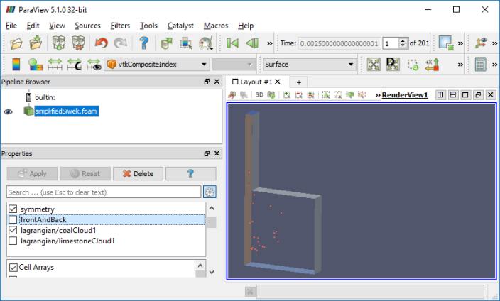
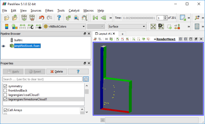
combustion >> coalChemistryFoam >> simplifiedSiwek: As per the source code, coalChemistryFoam is a transient solver for: [a] compressible, [b] turbulent flow with [I] coal and limestone parcel injections, [II] energy source and [III] combustion. The coal particles are injected as per specified positions mentioned in the file constant/coalCloud1Positions and constant/limestonePositions.
Types of Combustion
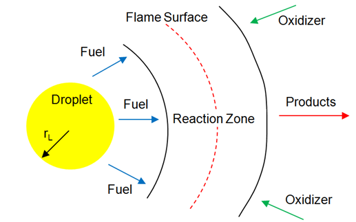
Non-Premixed Combustion
In this mode, molecular mixing of fuel and oxidizer plays a dominant role. The combustion zone has a distinct flame front where fuel and oxidizers are in stoichiometric ratio, though flame fronts do not have a characteristic velocity and do not propagate. They remain attached to the stoichiometric surface between the fuel and the oxidizer. The flame front surface itself may be transported (convected) from place to place by the local flow field. The mixture fraction is used to quantify local fuel/air ratio and solved as a (conserved scalar) field variable. Equations for individual species are not solved. Instead, species concentrations are derived from the predicted mixture fraction fields.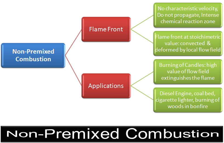
Excerpts from ANSYS Tutorials: "When you use the non-premixed combustion model, you need to create a PDF table. This table contains information on the thermo-chemistry and its interaction with turbulence. ANSYS Fluent interpolates the PDF during the solution of the non-premixed combustion model."
Examples includes jets, jets in cross- or co- or swirl-flows.Premixed Combustion
Since fuel and oxidizer are already mixed, molecular mixing does not influence combustion phenomena. Unlike non-premixed combustion, the flame front propagates spontaneously with a characteristic velocity called the burning velocity in a direction normal to itself in order to consume the available reactant mixture. The flame front is the surface of discontinuity between the burnt and unburnt regions. Excepts from ANSYS FLUENT: "Premixed combustion is much more difficult to model than non-premixed combustion. The reason for this is that premixed combustion usually occurs as a thin, propagating flame that is stretched and contorted by turbulence. To capture the laminar flame speed, the internal flame structure would need to be resolved, as well as the detailed chemical kinetics and molecular diffusion processes. Since practical laminar flame thicknesses are of the order of millimeters or smaller, resolution requirements are usually unaffordable. The essence of premixed combustion modeling lies in capturing the turbulent flame speed, which is influenced by both the laminar flame speed and the turbulence."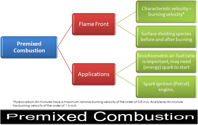
The calculation method for temperature depends on whether the model is adiabatic or non-adiabatic. ANSYS FLUENT has two options to model pre-mixed combustion.
| Premixed combustion model | Features |
| Adiabatic | Adiabatic Temperature of Burnt Products Tad, which is the temperature of the burnt products under adiabatic conditions needs to be specified. This temperature will be used to determine the linear variation of temperature in an adiabatic premixed combustion calculation: T = (1 − c) × Tu + c × Tad |
| Non-Adiabatic | For non-adiabatic models, the Heat of Combustion per unit mass of fuel and the Unburnt Fuel Mass Fraction need to be specified. The solver uses these values to compute the heat losses or gains due to combustion and include these losses/gains in the energy equation that it uses to calculate temperature. The Heat of Combustion can be specified only as a constant value, but one can specify either a constant value or use a UDF for the Unburnt Fuel Mass Fraction. |
Partially Premixed Combustion
Most of the practical applications are partially pre-mixed type. Applications are gas turbines and after-burners.
Excerpts from User Guide - ANSYS FLUENT: "Partially premixed combustion systems are premixed flames with non-uniform fuel-oxidizer mixtures (equivalence ratios). Such flames include premixed jets discharging into a quiescent atmosphere, lean premixed combustors with diffusion pilot flames and/or cooling air jets, and imperfectly mixed inlets. Behind the flame front (c = 1), the mixture is burnt and the equilibrium or laminar flamelet mixture fraction solution is used. Ahead of the flame front (c = 0), the species mass fractions, temperature and density are calculated from the mixed but unburnt mixture fraction. Within the flame (0 < c < 1), a linear combination of the unburnt and burnt mixtures is used."
Species Transport in ANSYS FLUENT
Typical bond strengths
Reference: Flagan and SeinfeldDiatomic molecules
| Bond | kJ/mol |
| H-H | 437 |
| H-O | 429 |
| H-N | 360 |
| C-N | 729 |
| C-O | 1076 |
| N-N | 950 |
| N-O | 627 |
| O-O | 498 |
Polyatomic molecules
| Bond | kJ/mol |
| H-CH | 453 |
| H-CH2 | 436 |
| H-CH3 | 436 |
| H-C2H3 | 436 |
| H-C2H5 | 411 |
| H-C3H5 | 356 |
| H-C6H5 | 432 |
| H-CHO | 385 |
| H-NH2 | 432 |
| H-OH | 499 |
| HC≡HC | 964 |
| H2C=CH2 | 699 |
| H3C-CH3 | 369 |
| O=CO | 536 |
The content on CFDyna.com is being constantly refined and improvised with on-the-job experience, testing, and training. Examples might be simplified to improve insight into the physics and basic understanding. Linked pages, articles, references, and examples are constantly reviewed to reduce errors, but we cannot warrant full correctness of all content.
Template by OS Templates