- CFD, Fluid Flow, FEA, Heat/Mass Transfer: Feedbacks/Queries -

Turbulence Modeling
Turbulence: a necessity! Why it needs to be modelled and how it is modelled?
Turbulence Modeling: Best Practice Guidelines
Sir Horace Lamb, 1932, in an address to the British Association for the Advancement of Science:"I am an old man now, and when I die and go to heaven there are two matters on which I hope for enlightenment. One is quantum electrodynamics, and the other is the turbulent motion of fluids. And about the former I am rather optimistic."
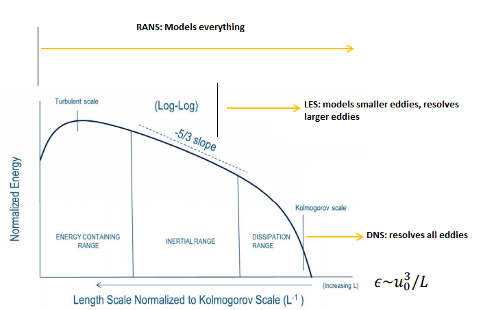
Despite such a remarkable and intriguing characteristics of "turbulent motion", there is no formal definition of turbulence and it has been characterized intuitively using terms like turbulent kinetic energy, turbulent dissipation rate and so on. One of the best known and a bit poetic definition is by Richardson which explain the energy cascade from mean flow to viscous dissipation at walls.
Big whorls have little whorls,
which feed on their velocity;
And little whorls have lesser whorls,
And so on to viscosity.
Note the term 'viscosity' here. As "laminar viscosity" governs the flow field in laminar flows, "turbulent viscosity" is required to find out flow field in turbulent flows. The basic purpose of any turbulence model is to estimate the "turbulent or eddy viscosity". In its algebraic form, it can be simply represented as proportional to product of a "turbulent velocity scale (VTURB)" and a "turbulent length scale (LTURB)". Thus, indirectly turbulence model is a method to estimate VTURB and LTURB since they are not known a-priori. Such methods are known as mixing-length or "Zero-Equation Models" which have limited application as the eddy viscosity becomes constant throughout the domain. This type of turbulence models do not have capability to predict separation and reattachment. This has led to development of other methods which can help estimate these flow scales. Reynolds Averaged Navier Stokes (RANS) equation is one of them. This method has led to many other variables such as k, ε and ω as well as transport equations governing them.
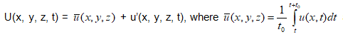
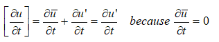
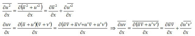
Let's see how a RANS is developed. The basic approach is to represent the spatially and time varying flow with a mean component varying spatially, u(x) and fluctuating component varying with space and time - known as Reynolds decomposition of u(x, t).
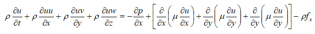
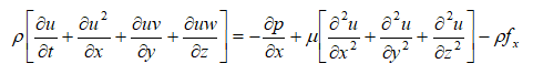

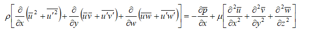
Note that the mathematical manipulation performed on Navier-Stokes (N-S) equation to derived RANS does not mean it is not applicable for turbulent flows. N-S equation is applicable to turbulent flows as good as it is for laminar flows. Statistical averaging is just a mathematical operation to reduce the computational effort (even an engineering attempt to make is feasible) albeit at a small impact on accuracy. In the following paragraphs, the terms associated with turbulence modelling, available methods and some recommendations have been described.
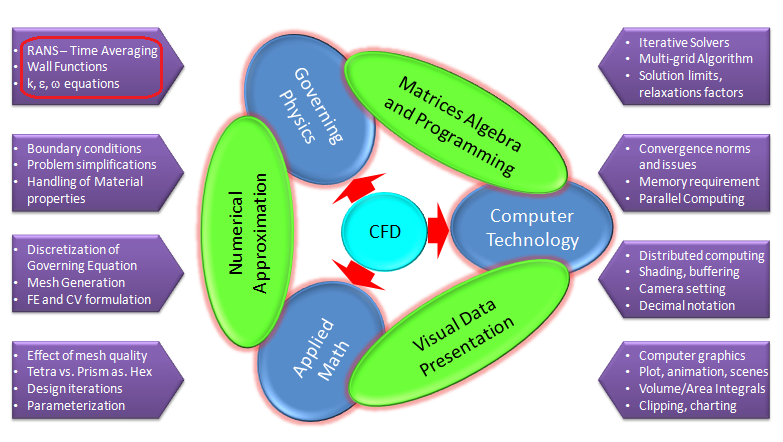
Before moving on the necessity of turbulence modelling, few words on the technologies involved in CFD simulations. Any numerical simulation program has to deal with governing physics and its numerical applications, conversion of partial differential equations into equivalent matrix form and using computer to let users visualize the inputs and outputs. The picture below summarizes the inter-dependence of technology and applied mathematics. "Turbulence modelling" is one of the most critical steps in overall simulation process: be it development of the program itself or application to real-life problems.
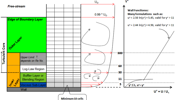
This page deals with the concept of turbulence and how it is mathematically represented in CFD simulation programs. Walls are main source of vorticity and turbulence and its presence gives rise to turbulent momentum and thermal boundary layers: accurate prediction of frictional drag for external flows and pressure drop for internal duct flows depends on accuracy of local wall shear stress predictions. In this context, the steep variations of field variables (velocity, temperature ad pressure) are in the very near-wall regions shown by following picture.
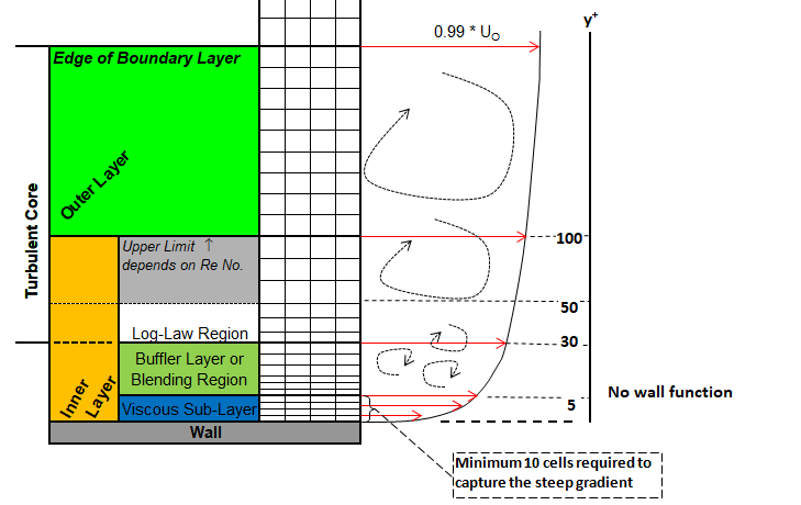
The zone near the walls are known as boundary layer and has further been divided into sub-layers. Turbulence and boundary layer are two very closely related topics. While overall flow is divided into two zones: boundary layer and free-stream, boundary layers themselves are divided into 4 zones: viscous sub-layer, buffer-layer, log-law region and outer layer. Log-law region is also called "inertial sublayer". Outer layer is also known as "defect layer". Log-region and inertial sublayer is sometimes collectively called "overlap layer".
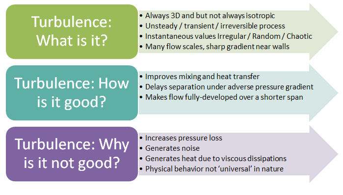
Use of very fine mesh to resolve these steep profiles is in most of the applications computationally too expensive for application of CFD tools to the industrial scale. Hence, special near-wall treatments have been developed since governing equations cannot be integrated down to wall. This led to the evolution of wall functions and near wall treatment. But turbulence is not an undesirable thing under all circumstances. The image describes the features of "turbulent motions" as well as few of the benefits too.
The complicated turbulent motion is the result of the non-linear advection that creates interactions between different scales of motion. The large scales are governed by the geometrical scales and the smallest scale, known as Kolmogorov scale, is constrained by the viscosity of the fluid.
- Though all fluid flows are governed by Navier-Stokes equations, the wide range of length and time scales poses difficulties in treating turbulence, both analytically and numerically. Statistically large number of length scales also cause non-repeatibility where calculations tend to be sensitive to initial conditions and turbulence level at the inlet boundary.
- The presence of too may flow scales demands computational resources too high for most industrial applications. To address this, the governing equations are either time/spatially filtered to remove all/some of the turbulent scales.
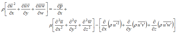
- This approach results in a tractable set of equations for numerical calculations, closure problem arises from the correlated velocity fluctuations as explained above in derivation of Reynolds stresses. So, a turbulence model is needed to represent the effect of the small scales on the mean flow.
- There are no unique turbulence model that fits all the requirements. k-ε model is the workhorse of the industry but needs to be used with caution. k-ω SST generally gives good results in most of the cases where k-ε fall short. Yet one must investigate the effect of different turbulence models for the particular case being investigated.
Last but not the least, an excerpts from Academic Resource Center of Illinois Institute of Technology:
"The phenomenon of turbulence, caused by the convective terms, is considered the last unsolved problem of classical mechanics. We know more about quantum particles and supernova than we do about the swirling of creamer in a steaming cup of coffee!"
Key Parameters for Specification of Turbulence
- Energy cascade: Cascade refers to a "transfer process". In turbulent flows, it refers to the transfer of kinetic energy from large scales of motion, through successively smaller scales, ending with viscous dissipation and conversion to heat.
- Ergodicity and Homogeneous Turbulence: Ergodiity refers to the case when time averages and ensemble averages are equivalent. Homogeneous turbulence is when statistical properties do not change with spatial translation (turbulent behaviour do not change with position).
- Auto-correlations, cross-correlations, intermittency and stochastic (variable whose auto-correlation decays to zero exponentially) are few other terms used to define turbulence and its attributes.
- Vorticity: This is neither a physical property of the fluid nor a directly measurable physical characteristics (like velocity or pressure) of the flow field. It is a mathematical definition where vorticity ω = ∇ × V.
- Friction Velocity: This is a velocity scale to define the wall shear stress and designated as u* = (τW/ρ)1/2. This parameter is used to calculate y+ value explained below.
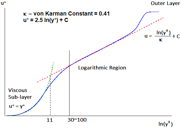
- Dimensionless Velocity: This is the ratio of local velocity scale to the friction velocity: u+ = u/u*. Note in the viscous sub-layer, velocity varies approximately linearly with the height y perpendicular to the wall. The need to have a dimensionless velocity to represent it as function of y+ which is a dimensionless number. This function is known as law-of-the-wall.
- y-plus or y+: First and the foremost, its definition is analogous to the Reynolds number. Similar to mean flow Reynolds number which defines the laminar, transition and turbulent flow regime, y+ can be thought as the number which defines the zone or height of layer dominating viscous dissipation, zone with balance of turbulent production and dissipation and finally the zone where turbulent production exceeds dissipation. Mathematically, y+ = ρu*y/μ where y is the height normal to the wall. Thus:
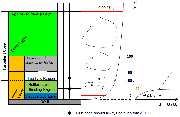
- 0 ≤ y+ ≤ [5~11]: Viscous sub-layer. There is no unique value agreed upon in the industry on upper layer of viscous sub-layer. As per Lienhard[4], the upper boundary of viscous sub-layer is ≅ 7.
- [5~11] ≤ y+ ≤ 30: Buffer layer
- 30 ≤ y+ ≤ 100: Log-layer. Note that the upper boundary of log-layer varies for flow types and typically a value of y+ ≤ 100 is industry accepted limit.
- y-star or y*: In ANSYS FLUENT, the laws-of-the-wall for mean velocity and temperature are based on the wall unit y* rather than y+. The definition of y* uses u* instead of u+ where y* = ρCμ1/4k1/2y/μ and u* = ρCμ1/4k1/2/τW. These two quantities are approximately equal in equilibrium turbulent boundary layers.
- Turbulent (or Eddy) Viscosity: μt and Eddy Diffusivity εm for Momentum
- Analogous to molecular viscosity, turbulence viscosity is related to fluctuating component of the velocity. It is the constant of proportionality between turbulent (Reynolds) stresses and mean (large-scale) strain rate, analogous to laminar viscosity in Newton’s law of viscosity.
- Molecular viscosity is a property of the fluid where as eddy viscosity is property of the flow field more than the property of the fluid
- μt = Cμ * ρ * k2 / ε where Cμ = 0.09, an empirical coefficient.
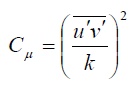 Measurements in equilibrium flows (production = dissipation) suggest that Cμ ~ 0.09.
 - Since u', v' and w' are not modelled in CFD except DNS approach, how do we estimate u' and k? The answer is Boussinesq hypothesis: which relates the Reynolds stresses to the mean velocity gradients. This hypothesis is used in Spalart-Allmaras model, k-ε and k-ω models.
- Boussinesq hypothesis: Turbulent viscosity is expressed based on analogy with molecular transport of momentum [viscous stresses are linearly proportional to mean strain rates]- hence assumptions is valid at molecular level, not necessarily always valid at macroscopic level.
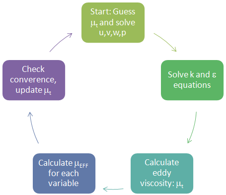
Thus, calculation of a turbulent flow using eddy viscosity model for turbulence will follow the cycle described below.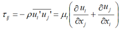
- Thermal Diffusivity, γ: Molecular transport of scalar quantities (such as heat and species) is analogous to the transport of momentum. Thus, heat flux is a sum of the contributions of the "heat transport by molecular motion" and "heat transport due to the turbulent motion". Note that Prandtl number is ratio of eddy diffusivity of momentum and eddy diffusivity of heat (thermal diffusivity). This analogy is valid when Prandtl number is close to 1 which is true for most of the gases.
- Turbulent Intensity: I
- The turbulent intensity I, is defined as the ratio of the root-mean-square of the velocity fluctuations u', to the mean flow velocity, umean. For pipe flow, I=0.16 / ReDH1/8 - the value of TI at different values of Reynolds number are Re=[2000, 5000, 10000, 50000, 100000, 500000] : TI=[0.0619, 0.0552, 0.0506, 0.0414, 0.0379, 0.0310]
- A turbulent intensity of 1% or less is generally considered low and turbulent intensities greater than 10% are considered high.
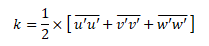
- Turbulent Kinetic Energy: k [m2/s2]
- It is specific (per unit mass) kinetic energy of eddies = 1/2 * v'2
- This is trace of Reynolds stress tensor, computed by summing the diagonals of the matrix of components. Thus, TKE,
- It defines velocity scale of the turbulence (eddies). Remember Ryenolds number is ratio of [length scale] * [velocity scale] / [kinematic viscosity]
- k = 3/2 * [UMEAN * I]2 and at 10 [m/s] and I = 0.1%, k = 1.5E-4 [m2/s2] and at 1 [m/s], k = 1.5E-6 [m2/s2]
- Turbulent Eddy Dissipation Rate: ε = -dk/dt [m2/s3]
- It is rate of conversion of k into heat or thermal energy per unit mass. ω = ε/Cμ/k and eddy viscosity νt = k/ω
- Along with k, it defines length scale of the flows (turbulent eddies)
- From dimensional arguments, ε = Cμ0.75 × k1.5/L where Cμ is an empirical constant = 0.09, and L is the length scale of turbulence producing eddies in the flow. At 1 [m/s], L = 1 [mm] and I = 0.1%, ε = 3.0E-7 [m2/s3].
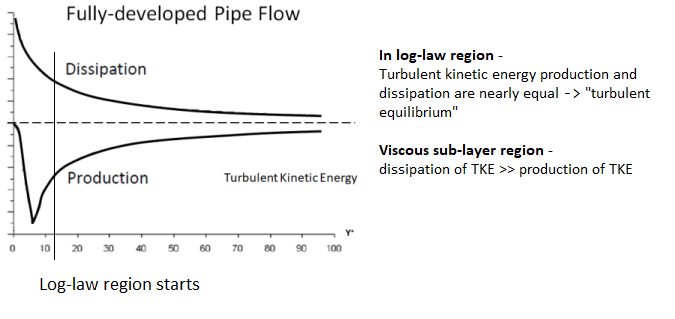
- Following plot described the production and dissipation of TKE. Note that k and ε are in almost equilibrium far away from the wall.
- Turbulent Eddy Dissipation Frequency: ω [s-1]
- It is rate of conversion of k into thermal energy per unit volume.
- It can be defined implicitly by k and ε, where ω = ε/Cμ/k = k0.5/[Cμ0.25 × L] where Cμ is an empirical constant = 0.09, and L is the length scale of turbulence producing eddies in the flow. L= 0.07 x D / Cμ0.75 where D is the hydraulic diameter.
- Flow scales: Also known as Kolmogorov ('dissipation') scales, it represents smallest (length, time and velocity) of turbulent fluctuations:
- (Kolmogorov) Length scale, η = (ν3 / ε)1/4 where ν is the kinematic viscosity in [m2/s]. The size of largest tubulent producing eddies are appriximated to be equal to the hydraulic diameter (also called as integral length scale).
- (Kolmogorov) Time scale, τ = (ν / ε)1/2
- (Kolmogorov) Velocity scale, u = (ν . ε)1/4
- Thus, it would required N = L/η = L×ε1/4/ν3/4 = Re3/4 cells to capture all the scales in one direction and thereby extrapolating for a 3D domain, the number of cells necessary to capture all scales is (Re3/4)3 = Re9/4, which for Reynolds numbers of the order of 105 will require ~1011 = approximately 100 billion cells.
- Summary: RANS methods
- Step-1: Mean flow velocity and pressure equations are solved.
- Step-2: TKE (k) and TED (ε) equations are solved.
- Step-3: Turbulent viscosity is solved using equations described above.
- Step-4: Reynolds stress tensor is modeled (estimated) using Boussinesq hypothesis.
Wall treatment and the wall functions
- "High-Re number wall treatment" refers to case where boundary layers are modelled in terms of empirical (and well-established) correlations known as wall functions. Wall laws are used to calculate wall shear stress. In the wall function model, the first node near the wall is assumed to lie outside of the log-law region that is y+ ≥ 30
- "Low-Re number wall treatment" refers to the case when boundary layers are resolved and not modeled. The Re-number here refers to Turbulent Reynolds Number defined as ReTURB = k2ν/ε.
- Note that it is related to the way boundary layers are resolved and has nothing to do with the "MEAN FLOW REYNOLDS NUMBER".
- A "low Reynolds number" turbulence model doesn't use wall functions, that is does not involve any assumptions about the near-wall variation of velocity.
- Examples include k-ω SST or low Reynolds number k-ε (a variant of k-ε that does not use wall functions and integrates right through the boundary layer).
- When "Low-Re number wall treatment" is used, following requirements on mesh are imposed:
- The (y+) should be of the order of 1.
- Under no circumstances, the y+ should increase above 5.
- The number of elements in the boundary layer should be ~ 10. This ensures that the mesh corresponding to y+ ≥ 30 falls in the log-law region.
- For all "high-Re number wall treatments" such as (a) scalable wall function [exploits a limiter in the (y+) calculations such that y+ = min [y+, 11.36] in CFX, (b) standard wall functions in FLUENT and (c) standard wall function in STAR-CCM+. Some literatures report 11.225 instead of 11.36.
- The centroid of cell adjacent to walls should lie in logarithmic region: y+ ≥ 30 in FLUENT and STAR CCM+ because they use cell-centred schemes (staggered arrangement).
- The nodes of 1st layer of elements should fall in y+ ≥ 30 in ANSYS CFX. This software uses vertex-centred scheme (collocated arrangement).
- A scalable wall function (SWF) is another way of saying wall surface coincides with the edge of the viscous sublayer if the first grid point is too close to the wall. Still other explanation is that scalable wall functions effectively shifts the near-wall mesh point to y+ = 11 regardless of the close it is to the wall. Thus, scalable wall functions can be assumed less sensitive to mesh as compared to standard or non-equilibrium wall functions but that does not imply they are necessarily more accurate.
- What happens if more than 1 layers of mesh are inside viscous layer - how does scalable wall function treat the second node falling inside viscous layer?
- No noticeable impact on result is likely even if the y+ falls up to the level of 11.36, in any "high-Re number wall treatments"
- It is not possible to maintain y+ value in a very narrow band. It is advised to target a y+ band of 30 ~ 50 for higher accuracy. A range of 30 ~ 100 on y+ yields result which is acceptable for design iterations.
- The y+ value should not be allowed to cross the upper limit of 300.
- It is not possible to maintain this limit (y+ > 11.36) in few areas of the fluid flow such as separation and stagnation (recirculation) zones. This is numerically acceptable and no impact of results should be anticipated because boundary layers are neither orderly nor as steep as normal wall-bounded turbulent flows with separations.
- There are "numerical improvisations" where the wall treatment toggles automatically between "Low-Re number wall treatment" and "high-Re number wall treatments". This is known as "automatic near-wall treatment" where wall treatment automatically switches from wall-functions to a low-Re formulation as the y+ value changes based on local mesh refinement.
- Enhanced Wall Treatment (EWT) or Enhanced Wall Functions (EWF): Blended law-of-the-wall are applied for momentum, energy, species and turbulent dissipation frequency. The blending function for momentum is of the form u+ = eΓ . u+LAM + 1/eΓ . u+TURB.
- EWT and SWF are expected to be insensitive to y+ among near wall modelling approaches.
- In other words, as the grid is refined or coarsened in certain range of y+, the results will not show strong dependence on grid resolution.
- EWT is also a "viscous sub-layer resolving approach". Thus, when used with a mesh that is fine enough to capture the flow behavior in the viscous sublayer (that is y+ < 1), the accuracy of results can be be expected to be better than with other wall function approaches.
- In a case where the nodes of the first layer of elements near the wall are always in the log-layer, no significant difference between EWT and scalable wall functions would be observed.
- FLUENT does not allow modelling of wall roughness with EWT. Scalable or standard wall function will need to be used to account for effect of surface roughness on shear stress and pressure drop.
- Law of the Wall:
- Friction Velocity: uτ = [τW/ρ]0.5, τW = wall shear stress, ρ = density of fluid
- Dimensionless Velocity: u+ = uτ / uY1, uY1 = Velocity at first node near wall and parallel to the wall
- There are many versions of the logarithmic law of the wall. One such example valid in the range 30 ≤ y+ ≤ 130 is: u+ = ln[E . y+ / κ], E = surface roughness parameter, equal to 8.6 for smooth walls and κ is von Karman constant = 0.41

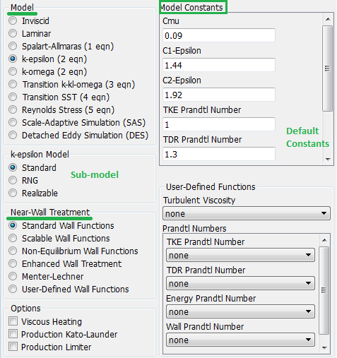
Realizable k-ε Model: Standard k-ε model derives a modeled equation for the dissipation (ε) using the k-equation as a starting point. The realizable k-ε model's equation originates from the exact transport equation of <ω'iω'i> where ω'i is the fluctuating vorticity. The k-equation remains same in both standard and realizable variants.
Stanadard k-ε model cannot universally ensure positive value of normal stresses and Schwarz’s inequality of shear stresses. Here equation for k remains same as standard k-ε model but the ε-equation is based on a transport equation for the mean-square vorticity fluctuation and Cμ is a function of mean velocity field and turbulence. It addressed the anomaly of standard k-ε model in round jet (jet emanating from a circular hole) and plane jet (jet emanating from a rectangular opening of high aspect ratio) and predicts the spreading rate correctly for both types of jets.
Classification of turbulence models
The term "Isotropic" refers to both Isotropic diffusion and Isotropic dissipation whereas in reality near-wall flows are anisotropic due to presence of walls. Imagine the flow perpendicular to the wall and near the wall - the fluctuations in direction perpendicular to the wall will slow-down faster in the direction parallel to it. In the following diagram, one-, two- and four-equation models refer to the number of additional partial differential equations required (beyond the equations for mean quantities u, v, w, p, T) to complete a RANS model.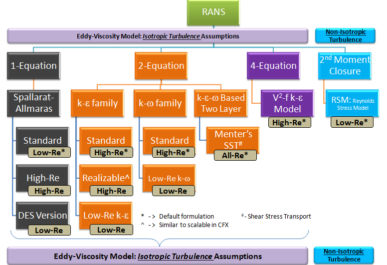
Characteristics of turbulence models
k-ε model: Velocity scale: k1/2, Length scale: k3/2/ε, Eddy viscosity: ρ Cμ k2/ε- Advantages:
- Good results for many industrial applications dealing with wall-bounded flows with low pressure gradients.
- Stable and numerically robust.
- Computationally less expensive, no sensitivity of free-steam conditions.
- Realizable version of k-ε model is good for complex flows with large strain rates, recirculation, rotation, separation, strong pressure gradients.
- Disadvantages:
- Limited ability to predict secondary flow characteristics such separation and reattachment (such as flow over aerofoil with non-zero angle of attack, cross flow over a cylinder).
- Not accurate in flows with high streamline curvature and sudden changes in the mean strain rate (such as back-facing step), strong swirling flow (such as cyclones, hydro-cyclones and stirred tanks).
- Like any eddy-viscosity model, fails to predict the cases where turbulence transport or non-equilibrium effects are important in flows. It is based on isotropic turbulence.
Spalart-Allmaras model
- Key characteristics:
- In standard form, it is a Low-Re number model and hence no wall function is used. That further imposes a restrictions to have mesh fine enough so that y+ is < 1.0 everywhere.
- Since this is a Low-Re number model, it can be used with "Automatic Wall Treatment" or "All y+ treatment" methods of turbulence modelling.
- This turbulence model had especially been developed for aerodynamic flow simulation for aerospace industry.
- This models is a good choice for applications in which the boundary layers are largely attached and separation is not present or mild separation is expected. Typical examples would be flow over a wing, ship-hulls, missiles, fuselage or other aerospace external-flow applications.
- The Spalart-Allmaras model for RANS equations is not recommended for flows dominated by free-shear layers (such as jets), flows where complex recirculation occurs (especially with heat transfer) and natural convection.
- The Spalart-Allmaras models with DES can be used for flows dominated by free-shear layers (such as jets), flows where complex recirculation occurs (especially with heat transfer) and natural convection.
Reynolds Stress Model (RSM) or Second Moment Closure Methods
- Key characteristics:
- Reynolds stresses are not modelled as Boussinesq Hypothesis. However, modeling is still required for many terms in the transport equations.
- Recommended for complex 3-D turbulent flows with large streamline curvature and swirl, but the model is computationally intensive, difficult to converge than eddy-viscosity models such as k-ε or Spalart-Allmaras models.
- Anisotropy of turbulence is accounted for, quadratic pressure-strain option improves performance for many basic shear flows.
- Most suitable for curved ducts say U or S-bends, rotating flow passages, combustors with large inlet swirl and cyclone separators.
Standard k-ω Model (SKO): Velocity scale: k1/2, Length scale: k1/2/Cμω, Eddy viscosity: ρ k2/ω
- Key characteristics:
- Specific dissipation rate ω = k/ε solved instead of ε
- Demonstrates better performance for wall bounded and low-Re flows and potential to handle transitional flows (though tend to predict the transition early).
- Suitable for complex boundary layer flows with adverse pressure gradient and separation (external aerodynamics and turbomachinery).
- Separation is typically predicted to be higher and earlier than experimentally observed values.
Shear Stress Transport (SST) k-ω Model
- Key characteristics:
- Specific dissipation rate ω = k/ε solved in inner layer (log-layer and viscous sub-layer) and transitions to a k-ε model away from the wall (but not same as standard k-ε equations).
- The boundary conditions for SST model are the same as the k-ω model and is relatively less sensitive to the free stream value of ω.
- Suitable for complex boundary layer flows with adverse pressure gradient and separation (external aerodynamics and turbomachinery).
Large Eddy Simulation (LES):
- Key characteristics:
- This model resolves all eddies with scales larger than grid scale and hence recommended for wide-band aeroacoustic noise predictions.
- Time step size is governed by the time scale of the smallest resolved eddies which requires the local Courant-Friedrichs-Lewy (CFL) number to order of 1.
- In ANSYS FLUENT, inlet perturbations at velocity inlets can be imposed while using LES turbulence model.
- FLUENT also recommends "Bounded Central Differencing" for momentum in case of LES on unstructured mesh.
References
- User manuals of commercial programs like FLUENT, CFX, STAR-CCM+
- Biswas Gautam, Som S. K., Chakraborty Suman: Introduction to Fluid Mechanics and Fluid Machines, Mc Graw Hill Education, Third Edition, 2012
- J. H. Ferziger and M. Peric’: Computational Methods for Fluid Dynamics, 4th Edition, Springer, Berlin, 2002
- John H. Lienhard IV and John H. Lienhard V: A Heat Transfer Textbook, 3rd Edition
- Introductory Lectures on Turbulence: Physics, Mathematics and Modeling by J. M. McDonough, Departments of Mechanical Engineering and Mathematics, University of Kentucky
The content on CFDyna.com is being constantly refined and improvised with on-the-job experience, testing and training. Examples might be simplified to improve insight into the physics and basic understanding. Linked pages, articles, references and examples are constantly reviewed to reduce errors, but we cannot warrant full correctness of all content.
Template by OS Templates