- ParaView: Open-source Post-Processor
WRITE YOUR OWN SOLVER
ParaView: Open-source Post-Processor
ParaView for OpenFOAM
Disclaimer:
This content is not approved or endorsed by OpenCFD Limited, the producer of the OpenFOAM software and owner of the OpenFOAM and OpenCFD trademarks.Excerpt from Tutorial: "ParaView is an open-source application for visualizing two- and three-dimensional data sets. The size of the data sets ParaView can handle varies widely depending on the architecture on which the application is run. The platforms supported by ParaView range from single-processor workstations to multiple-processor distributed-memory supercomputers or workstation clusters. ParaView comes with a pvpython application that allows you to automate the visualization and post-processing with Python scripting. The Visualization Toolkit (VTK) provides the basic visualization and rendering algorithms. VTK incorporates several other libraries to provide basic functionalities such as rendering, parallel processing, file I/O, and parallel rendering."
ParaView is written in C++. Wrappers exists for Java, Tcl and Python. pvpython is the Python interpreter that runs ParaView’s Python scripts in interactive or GUI mode. You can think of this as the equivalent of the paraview for scripting. pvbatch is also a Python interpreter that runs Python scripts for ParaView for batch processing.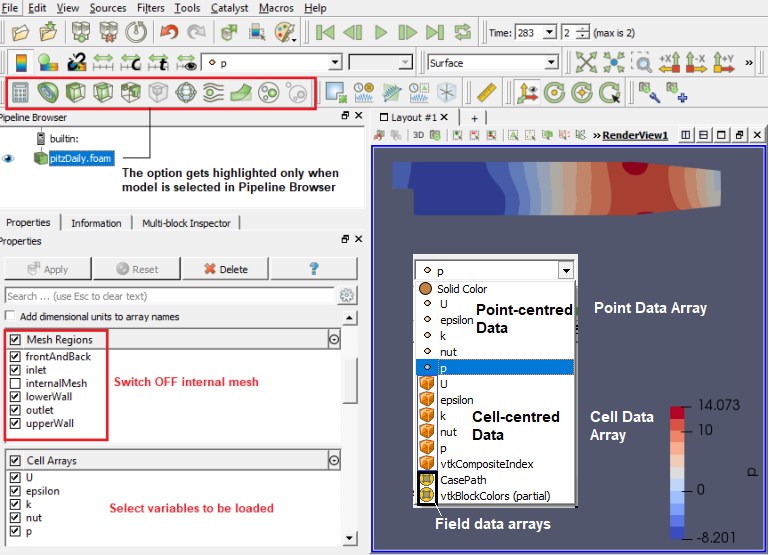
ParaView follows concept of blocks which refers to fluid zone, solid zone, boundary names. Individual surfaces are referred to as patched. It uses 'Source' and 'Filters' as post-processing operation. The tree starts with an input 'source' and filters can be added in parallel or parallel/series sequence.
The image above describes node-centred (or point-centred) and cell-centred schemes. Note that cell-centered attributes are assumed to be constant over each cell where as attribute is only defined on the vertices in a node-centred variable. Due to this property, many filters may not be directly applied to cell-centered attributes. It is normally required to apply a Cell Data to Point Data filter. Partial arrays is a term used to refer to arrays that are present on some non-composite blocks or leaf nodes in a composite dataset, but not all.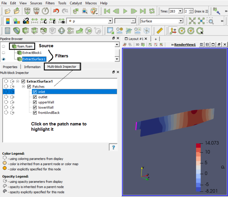
Reading Data from FLUENT and STAR-CCM+
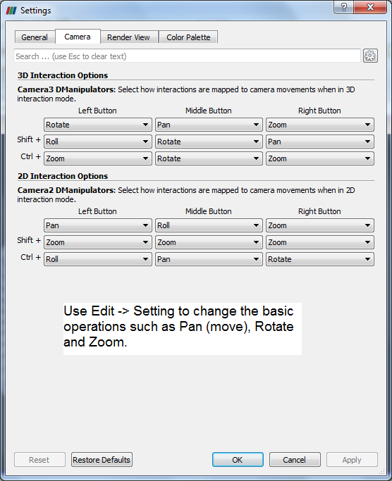
ParaView has the option to read the ANSYS FLUENT *.cas file and it can read only the cas file, *dat files cannot be read or loaded. Similarly, *.sim files from Simcentre STAR-CCM+ cannot be read directly into ParaView. The option is to export the FLUENT or STAR-CCM+ data in Ensight (Gold) format, *.case file. In ParaView, *.case file can be read with mesh topology as well as simulation result data. However, this option is applicable to only steady state results.The mouse operations to navigate can be set as shown in the following image.
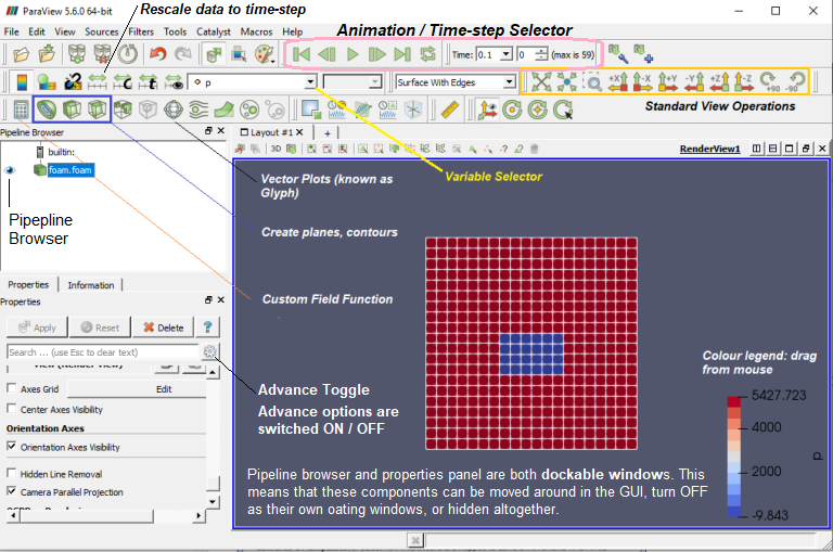
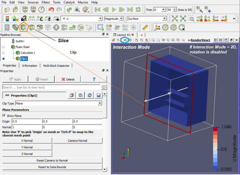
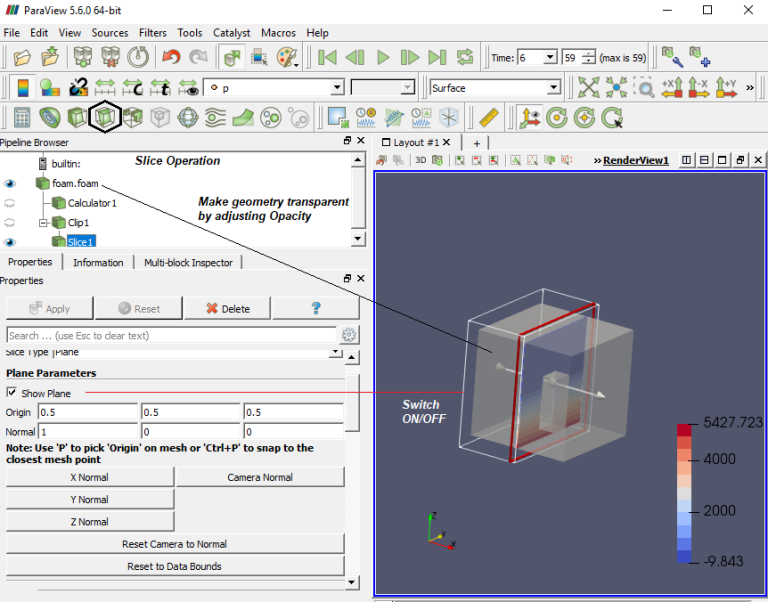
Paraview used filters which are functional units that process the data to generate, extract or derive features from the data. Filters are attached to readers, sources or other filters to modify its data in some way. These filter connections form a visualization pipeline. Use the p key to place alternating points, Ctrl+p places at nearest mesh point. Use the numeric 1 or 2 key to place the start or end point, Ctrl+1 or Ctrl+2 places at mesh point.
Drag the endpoints: use x, y or z key to constrain to axis. Press the key again to deactive the ortho-control.
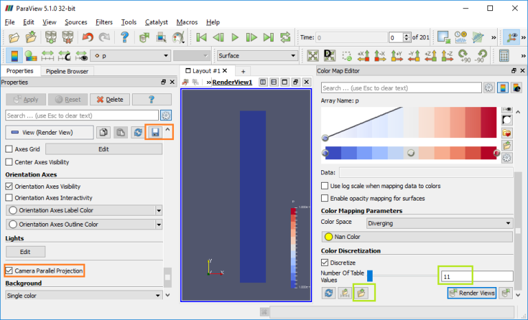
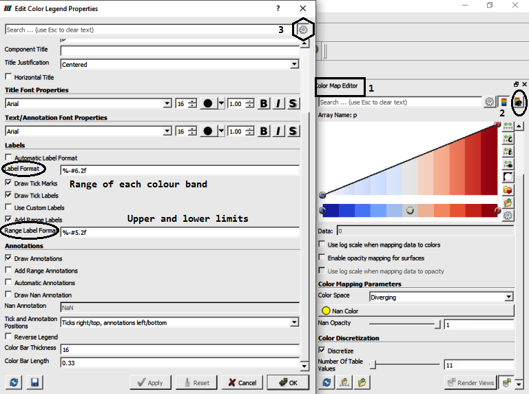
Set number format of the legend (color bar):
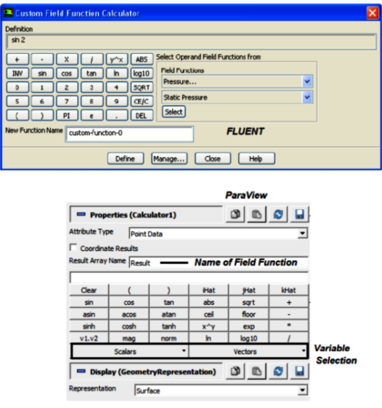
Vector plots and streamlines filters: Glyph Places a glyph, a simple shape, on each point in a mesh. The glyphs may be oriented by a vector and scaled by a vector or scalar. Stream Tracer Seeds a vector field with points and then traces those seed points through the (steady state) vector field. One important difference with respect to other post-processors is the way 'Contour' filter is defined in ParaView - here the contour filter computes isolines or isosurfaces using a selected point-centered scalar array. In prost-processors such as CFD-Post from ANSYS or STAR-CCM+ from Siemens, the 'contour' refers to a 2D plots on a specified plane or boundary surfaces.
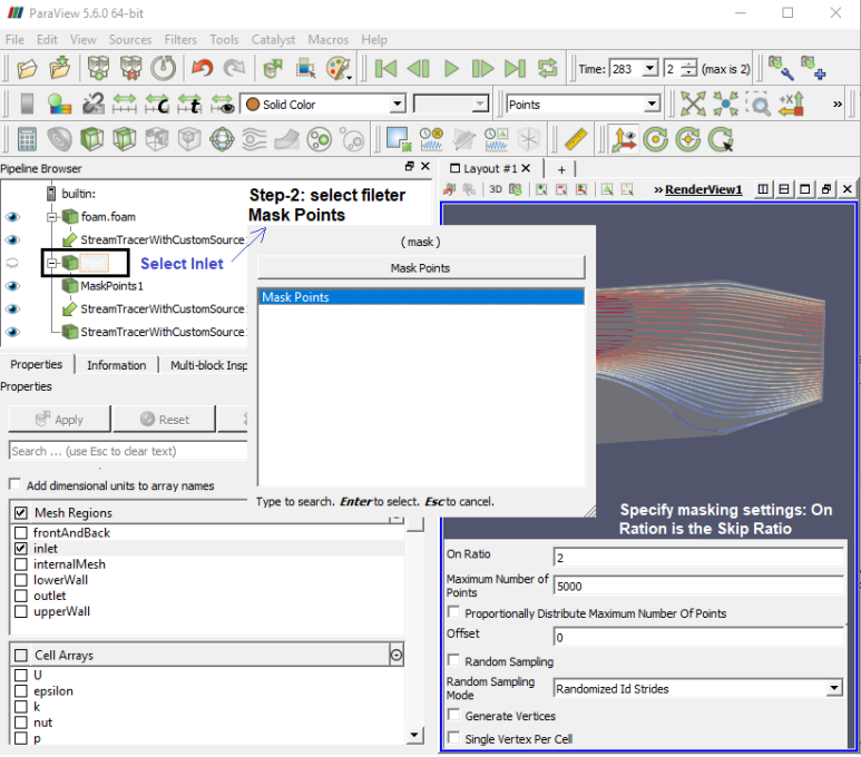
Mask Points (MaskPoints): Reduce the number of points. This filter is often used before glyphing. Generating vertices is an option. OnRatio: The value of this property specifies that every OnStride-th points will be retained in the output when not using Random (the skip or stride size for point ids). For example, if the on ratio is 3, then the output will contain every 3rd point, up to the the maximum number of points.
Cell Centers (CellCenters): Create a point (no geometry) at the center of each input cell.
Tube: Convert lines into tubes. Normals are used to avoid cracks between tube segments.
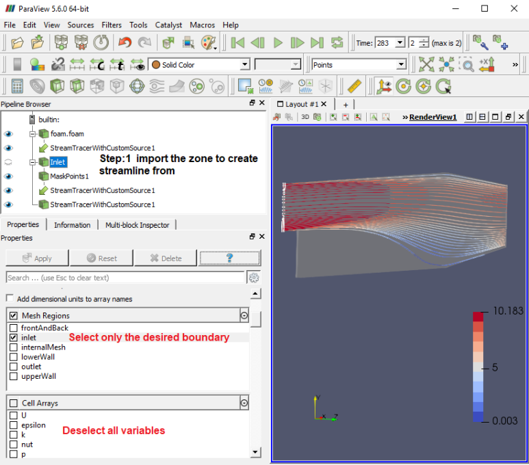
Steps to create streamline from a given boundary face:
Step-1
Step-2
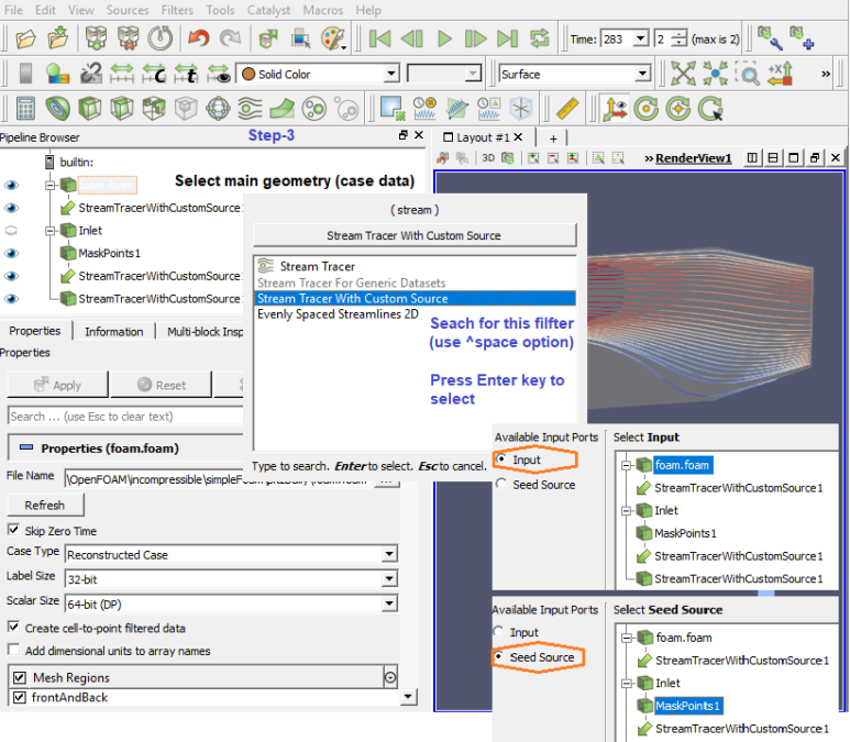
Step-3
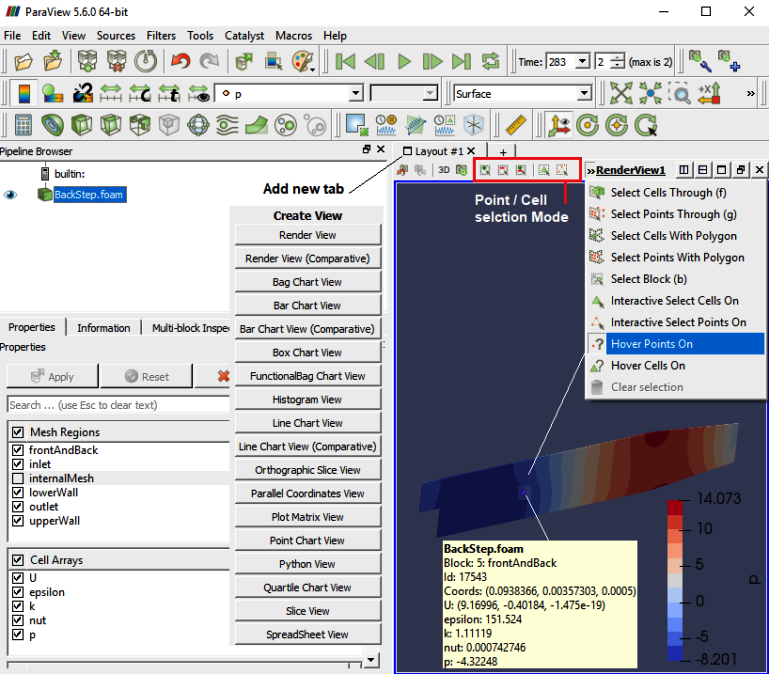
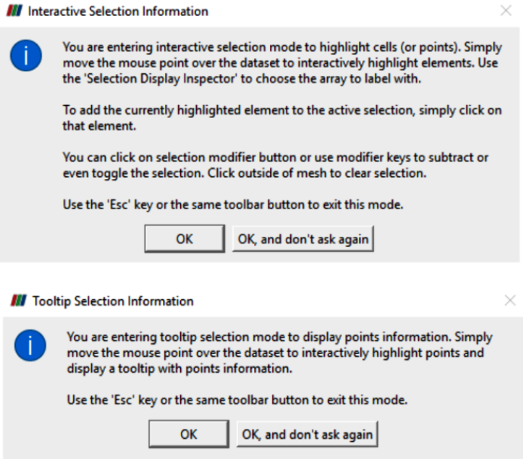
Paraview has interactive mode option to select cells and points. Hovering mouse over the points and cells will give relevant data on-the-fly.
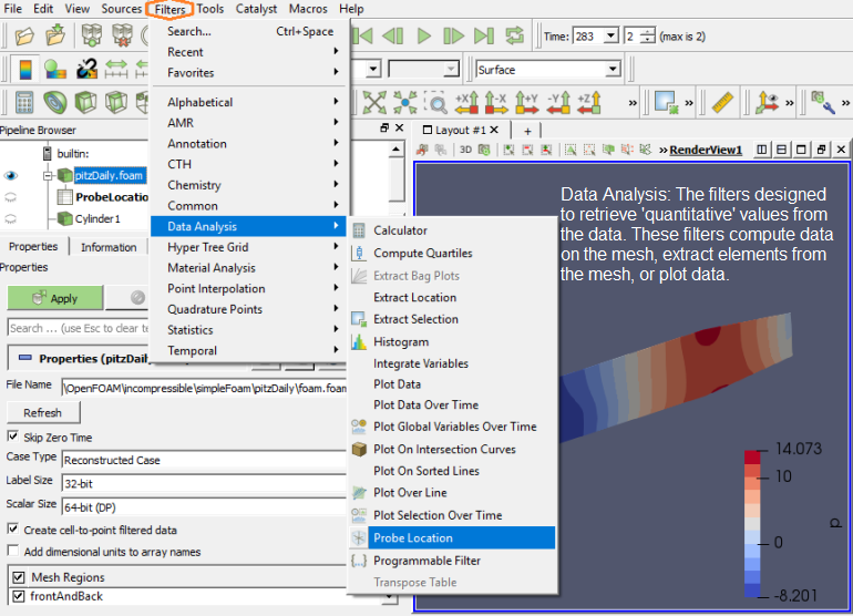
Extracting Data
To extract the selected elements and then save the result out as a new dataset or apply other filters only on the selected elements, then you need to use one of the "Extract Selection" filters. The Extract Selection and Plot Selection Over Time filters fall in this category of filters. This filter extracts a set of cells/points given a selection. The selection can be obtained from a rubber-band selection (either cell, visible or in a frustum) or threshold selection and passed to the filter or specified by providing an ID list. 
Compute Drag and Lift Forces due to Pressure
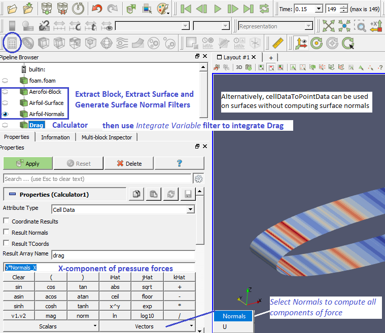
Extract Surface: When you apply the Extract Surface Filter, you will once again see the surface of the mesh. Although it looks like the original mesh, it is different in that this mesh is hollow whereas the original mesh was solid throughout. If you were showing the results of the contour filter, you cannot see the contour any more (after Extract Surface was applied). However, it is still in there hidden by the surface which can be viewed by appropriately hiding filters in "Pipeline Browser".
"Generate Surface Normals" requires a vtkPolyData as input which can be generated using Filter "Extract Surface". This data is used to generate surface normals. Filter "Gradient Of Unstructured DataSet" on a scalar results in a vector. One need to compute the velocity magnitude first and store it as a variable before trying to compute the gradient. You can do this using the calculator with a function 'mag(U)' naming it something like say 'Umag', then selecting 'Umag' as input to the 'Gradient' filter.
Similarly, to compute the dot product of two vectors, in the 'Calculator' it is simply '(Normals).(gradUmag)' where gradUmag is the gradient of Umag calculated in previous step. The "Compute Derivatives" filter takes point scalars and computes the gradient in the centroid of each cell (thus producing cell data). The 'Gradient' filter can take point data and find the data at the points or take cell data and find (an estimate of) the gradient at the cell centroids.
To visualize the Lagrangian particles the case must be converted into the ParaView format. The user should run the application foamToVTK on the case containing the Lagrangian Particle Tracking (LPT). This command will generate an additional folder named VTK inside the case directory. The case can be opened clicking on the file menu, open, and selecting the VTK directory. By clicking on the *.vtk file the case will be opened. The user must then open the files contained in the Lagrangian directory inside the VTK folder.
Python Script Example
Note that Python is case-sensitive.from paraview.simple import *
sphereInstance = Sphere ()
sphereInstance.Radius = 1.0
sphereInstance.Center [1] = 1.0
print(sphereInstance.Center)
sphereDisplay = Show( sphereInstance )
view = Render()
sphereDisplay.Opacity = 0.5
GetDisplayProperty ("Opacity")
Render(view)
Manipulate display properties
 readerRep = GetRepresentation()
 readerRep.DiffuseColor = [0, 0, 1]
 readerRep.SpecularColor = [1, 1, 1]
 readerRep.SpecularPower = 128
 readerRep.Specular = 1
 Render()
Manipulate view properties
 view = GetActiveView()
 view.Background = [0, 0, 0]
 view.Background2 = [0, 0, 0.6]
 view.UseGradientBackground = True
 Render()
Save Data and Screen-capture of Pots
 plot = PlotOverLine()
 plot.Source.Point1 = [0,0,0]
 plot.Source.Point2 = [0,0,10]
 writer = CreateWriter('⟨path⟩/plot.csv')
 writer.UpdatePipeline()
 plotView = CreateView('XYChartView')
 Show(plot)
 Render()
 SaveScreenshot('plotFile.png')
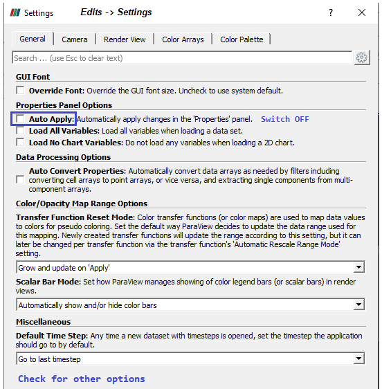
In Paraview, every time you hit Apply or change a display property, the UI automatically re-renders the view. In the scripting environment, you have to do this manually by calling the Render function every time you want to re-render and look at the updated result. Render function can take in an optional view argument, otherwise it simply uses the active view.
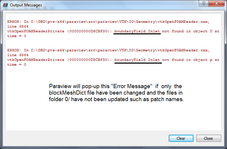
The names of patches defined in blockMeshDict needs to be same in files in folder 0/, otherwise ParaView will pop-up a warning message as shown below, if one wants to review the mesh only (after blockMesh command).
List of Filters in ParaView
| Name | Description |
| AMR Connectivity | Adaptive Mesh Refinement Fragment Identification |
| AMR Contour | Iso surface cell array. |
| AMR CutPlane | Planar Cut of an AMR grid dataset |
| AMR Dual Clip | Clip with scalars. Tetrahedra. |
| AMR Fragment Integration | Fragment Integration |
| AMR Fragments Filter | Meta Fragment filter |
| Add Field Arrays | Reads arrays from a file and adds them to the input data object. |
| Aggregate Dataset | This filter aggregates a dataset onto a subset of processes. |
| Angular Periodic Filter | This filter generate a periodic multi-block dataset. |
| Annotate Attribute Data | Adds a text annotation to a Render View |
| Annotate Global Data | Filter for annotating with global data (designed for Exodus II reader) |
| Annotate Time Filter | Shows input data time as text annotation in the view. |
| Append Arc-Length | Appends Arc length for input poly lines. |
| Append Attributes | Copies geometry from first input. Puts all of the arrays into the output. |
| Append Datasets | Takes an input of multiple datasets and output has only one unstructured grid. |
| Append Geometry | Takes an input of multiple poly data parts and output has only one part. |
| Append Molecule | Appends one or more molecules into a single molecule. |
| Block Scalars | The Level Scalars filter uses colors to show levels of a multi-block dataset. |
| Bounding Ruler | Create a line along the input to use as a ruler |
| Calculator | Compute new attribute arrays as function of existing arrays. |
| Cell Centers | Create a point (no geometry) at the center of each input cell. |
| Cell Data to Point Data | Create point attributes by averaging cell attributes. |
| Cell Size | This filter computes sizes for 0D (1 for vertex and number of points in for polyvertex), 1D (length), 2D (area) and 3D (volume) cells. Refer below for other options. |
| Clean | Merge coincident points if they do not meet a feature edge criteria. |
| Clean Cells to Grid | This filter merges cells and converts the data set to unstructured grid. |
| Clean to Grid | This filter merges points and converts the data set to unstructured grid. |
| Clip | Clip with an implicit function (an implicit description). Clipping does not reduce the dimensionality of the data set. The output data type of this filter is always an unstructured grid. |
| Clip Closed Surface | Clip a polygonal dataset with a plane to produce closed surfaces |
| Clip Generic Dataset | Clip with an implicit plane, sphere or with scalars. Clipping does not reduce the dimensionality of the data set. This output data type of this filter is always an unstructured grid. |
| Compute Derivatives | This filter computes derivatives of scalars and vectors. |
| Compute Molecule Bonds | Compute the bonds of a molecule based on interatomic distance only. |
| Compute Quartiles | Compute the quartiles table from a dataset or table. |
| Connectivity | Mark connected components with integer point attribute array. |
| Contingency Statistics | Compute a statistical model of a dataset and/or assess the dataset with a statistical model. |
| Contour | Generate isolines or isosurfaces using point scalars. |
| Contour Generic Dataset | Generate isolines or isosurfaces using point scalars. |
| Convert AMR dataset to Multi-block | Convert AMR to Multiblock |
| Convert Into Molecule | Convert a point set into a molecule. |
| Count Cell Faces | Counts the number of faces on each cell and appends a new cell data array. |
| Count Cell Vertices | Counts the number of vertices on each cell and appends a new cell data array. |
| Curvature | This filter will compute the Gaussian or mean curvature of the mesh at each point. |
| D3 | Repartition a data set into load-balanced spatially convex regions. Create ghost cells if requested. |
| Decimate | Simplify a polygonal model using an adaptive edge collapse algorithm. This filter works with triangles only. |
| Decimate Polyline | Reduce the number of lines in a polyline by evaluating an error metric for each vertex and removing the vertices with smaller errors first. |
| Delaunay 2D | Create 2D Delaunay triangulation of input points. It expects a vtkPointSet as input and produces vtkPolyData as output. The points are expected to be in a mostly planar distribution. |
| Delaunay 3D | Create a 3D Delaunay triangulation of input points. It expects a vtkPointSet as input and produces vtkUnstructuredGrid as output. |
| Descriptive Statistics | Compute a statistical model of a dataset and/or assess the dataset with a statistical model. |
| Name | Description |
| Distribute Points | Fairly distribute points over processors into spatially contiguous regions. |
| Elevation | Create point attribute array by projecting points onto an elevation vector. |
| Environment Annotation | Allows annotation of user name, date/time, OS, and possibly filename. |
| Evenly Spaced Streamlines 2D | Produce evenly spaced streamlines in a 2D vector field. |
| Extract AMR Blocks | This filter extracts a list of datasets from hierarchical datasets. |
| Extract Bag Plots | Extract Bag Plots. |
| Extract Block | This filter extracts a range of blocks from a multi-block dataset. |
| Extract CTH Parts | Create a surface from a CTH volume fraction. |
| Extract Cells By Region | This filter extracts cells that are inside/outside a region or at a region boundary. |
| Extract Component | This filter extracts a component of a multi-component attribute array. |
| Extract Edges | Extract edges of 2D and 3D cells as lines. |
| Extract Enclosed Points | Extract points inside a closed polygonal surface |
| Extract Generic Dataset Surface | Extract geometry from a higher-order dataset |
| Extract Level | This filter extracts a range of groups from a hierarchical dataset. |
| Extract Location | Sample or extract cells at a point. |
| Extract Region Surface | Extract a 2D boundary surface using neighbor relations to eliminate internal faces. |
| Extract Selection | Extract different type of selections. |
| Extract Subset | Extract a subgrid from a structured grid with the option of setting subsample strides. |
| Extract Surface | Extract a 2D boundary surface using neighbor relations to eliminate internal faces. |
| Extract Time Steps | Extract time steps from data. |
| FFT Of Selection Over Time | Extracts selection over time and plots the FFT |
| Feature Edges | This filter will extract edges along sharp edges of surfaces or boundaries of surfaces. |
| Gaussian Resampling | Splat points into a volume with an elliptical, Gaussian distribution. |
| Generate Ids | Generate scalars from point and cell ids. |
| Generate Quadrature Points | Create a point set with data at quadrature points. |
| Generate Quadrature Scheme Dictionary | Generate quadrature scheme dictionaries in data sets that do not have them. |
| Generate Surface Normals | This filter will produce surface normals used for smooth shading. Splitting is used to avoid smoothing across feature edges. |
| Ghost Cells Generator | Generate ghost cells for unstructured grids. |
| Glyph | This filter produces a glyph at points or cell centers in an input data set. The glyphs can be oriented and scaled by point or cell attributes of the input dataset. |
| Glyph With Custom Source | This filter produces a glyph at points or cell centers in an input data set. The glyphs can be oriented and scaled by point or cell attributes of the input dataset. |
| Gradient | This filter computes gradient vectors for an image/volume. |
| Gradient Of Unstructured DataSet | Estimate the gradient for each point or cell in any type of dataset. |
| Grid Connectivity | Mass properties of connected fragments for unstructured grids. |
| Group Datasets | Group data sets. |
| Group Time Steps | Group data set over time. |
| Histogram | Extract a histogram from field data. |
| Hyper Tree Grid - Axis Clip | Clip a HTG along an axis-aligned plane or box. |
| Hyper Tree Grid - Axis Cut | Cut a 3D HTG along an axis-aligned plane. |
| Hyper Tree Grid - Axis Reflection | Reflect an HTG across an axis-aligned plane. |
| Hyper Tree Grid - Cell Centers | Generate points at leaf node centers. |
| Hyper Tree Grid - Contour | Specialized Contour filter for HyperTreeGrid. |
| Hyper Tree Grid - Depth Limiter | Limit HTG nodes to a maximum depth |
| Hyper Tree Grid - Slice With Plane | Produce polydata describing a plane in the HTG. |
| Hyper Tree Grid - Threshold | Specialized Threshold filter for HyperTreeGrid. |
| HyperTreeGrid To UnstructuredGrid | Convert HyperTreeGrid to UnstructuredGrid. |
| Image Data To AMR | Converts certain images to AMR. |
| Image Data to Point Set | Converts an Image Data to a Point Set |
| Integrate Variables | This filter integrates cell and point attributes. |
| Interpolate to Quadrature Points | Create scalar/vector data arrays interpolated to quadrature points. |
| Intersect Fragments | The Intersect Fragments filter perform geometric intersections on sets of fragments. |
| Iso Volume | This filter extracts cells by clipping cells that have point scalars not in the specified range. |
| K Means | Compute a statistical model of a dataset and/or assess the dataset with a statistical model. |
| Level Scalars (Non-Overlapping AMR) | The Level Scalars filter uses colors to show levels of a hierarchical dataset. |
| Level Scalars (Overlapping AMR) | The Level Scalars filter uses colors to show levels of a hierarchical dataset. |
| Linear Extrusion | This filter creates a swept surface defined by translating the input along a vector. |
| Loop Subdivision | This filter iteratively divides each triangle into four triangles. New points are placed so the output surface is smooth. |
| Name | Description |
| Mask Points | Reduce the number of points. This filter is often used before glyphing. Generating vertices is an option. |
| Material Interface Filter | The Material Interface filter finds volumes in the input data containing material above a certain material fraction. |
| Median | Compute the median scalar values in a specified neighborhood for image/volume datasets. |
| Merge Blocks | Appends vtkCompositeDataSet leaves into a single vtkUnstructuredGrid |
| Mesh Quality | This filter creates a new cell array containing a geometric measure of each cell's fitness. Different quality measures can be chosen for different cell shapes. |
| Molecule To Lines | Convert a molecule into lines. |
| Multicorrelative Statistics | Compute a statistical model of a dataset and/or assess the dataset with a statistical model. |
| Normal Glyphs | Filter computing surface normals. |
| Outline | This filter generates a bounding box representation of the input. |
| Outline Corners | This filter generates a bounding box representation of the input. It only displays the corners of the bounding box. |
| Outline Curvilinear DataSet | This filter generates an outline representation of the input. |
| ParticlePath | Trace Particle Paths through time in a vector field. |
| ParticleTracer | Trace Particles through time in a vector field. |
| Pass Arrays | Pass specified point and cell data arrays. |
| Plot Data | Plot data arrays from the input |
| Plot Data Over Time | - |
| Plot Global Variables Over Time | Extracts and plots data in field data over time. |
| Plot On Intersection Curves | Extracts the edges in a 2D plane and plots them |
| Plot On Sorted Lines | The Plot on Sorted Lines filter sorts and orders polylines for graph visualization. |
| Plot Over Line | Sample data attributes at the points along a line. Probed lines will be displayed in a graph of the attributes. |
| Plot Selection Over Time | Extracts selection over time and then plots it. |
| Point Data to Cell Data | Create cell attributes by averaging point attributes. |
| Point Dataset Interpolator | - |
| Point Line Interpolator | - |
| Point Plane Interpolator | - |
| Point Volume Interpolator | - |
| Principal Component Analysis | Compute a statistical model of a dataset and/or assess the dataset with a statistical model. |
| Probe Location | Sample data attributes at the points in a point cloud. |
| Process Id Scalars | This filter uses colors to show how data is partitioned across processes. |
| Programmable Filter | Executes a user supplied python script on its input dataset to produce an output dataset. |
| Python Annotation | This filter evaluates a Python expression for a text annotation |
| Python Calculator | This filter evaluates a Python expression |
| Quadric Clustering | This filter is the same filter used to generate level of detail for ParaView. It uses a structured grid of bins and merges all points contained in each bin. |
| Random Attributes | This filter creates a new random attribute array and sets it as the default array. |
| Random Vectors | This filter creates a new 3-component point data array and sets it as the default vector array. It uses a random number generator to create values. |
| Rectilinear Data to Point Set | Converts a rectilinear grid to an equivalend structured grid |
| Rectilinear Grid Connectivity | Parallel fragments extraction and attributes integration on rectilinear grids. |
| Reflect | This filter takes the union of the input and its reflection over an axis-aligned plane. |
| Remove Ghost Information | Removes ghost information. |
| Resample AMR | Converts AMR data to a uniform grid |
| Resample To Image | Sample attributes using a 3D image as probing mesh. |
| Resample With Dataset | Sample data attributes at the points of a dataset. |
| Ribbon | This filter generates ribbon surface from lines. It is useful for displaying streamlines. |
| Rotational Extrusion | This filter generates a swept surface while translating the input along a circular path. |
| Name | Description |
| SPH Dataset Interpolator | - |
| SPH Line Interpolator | - |
| SPH Plane Interpolator | - |
| SPH Volume Interpolator | - |
| Scatter Plot | Creates a scatter plot from a dataset. |
| Shrink | This filter shrinks each input cell so they pull away from their neighbors. |
| Slice | This filter slices a data set with a plane. Slicing is similar to a contour. It creates surfaces from volumes and lines from surfaces. |
| Slice (demand-driven-composite) | This filter slices a data set with a plane. Slicing is similar to a contour. It creates surfaces from volumes and lines from surfaces. |
| Slice AMR data | Slices AMR Data |
| Slice Along PolyLine | Slice along the surface defined by sweeping a polyline parallel to the z-axis. |
| Slice Generic Dataset | This filter cuts a data set with a plane or sphere. Cutting is similar to a contour. It creates surfaces from volumes and lines from surfaces. |
| Slice With Plane | This filter slices a data set with a plane. Slicing is similar to a contour. It creates surfaces from volumes and lines from surfaces. This filter is faster than the standard Slice filter. |
| Smooth | This filter smooths a polygonal surface by iteratively moving points toward their neighbors. |
| StreakLine | Trace Streak lines through time in a vector field. |
| Stream Tracer | Integrate streamlines in a vector field. |
| Stream Tracer For Generic Datasets | Integrate streamlines in a vector field. |
| Stream Tracer With Custom Source | Integrate streamlines in a vector field. |
| Subdivide | This filter iteratively divide triangles into four smaller triangles. New points are placed linearly so the output surface matches the input surface. |
| Surface Flow | This filter integrates flow through a surface. |
| Surface Vectors | This filter constrains vectors to lie on a surface. |
| Synchronize Time | Set 'close' time step values from the source to the input |
| Table To Points | Converts table to set of points. |
| Table To Structured Grid | Converts to table to structured grid. |
| Temporal Cache | Saves a copy of the data set for a fixed number of time steps. |
| Temporal Interpolator | Interpolate between time steps. |
| Temporal Particles To Pathlines | Creates polylines representing pathlines of animating particles |
| Temporal Shift Scale | Shift and scale time values. |
| Temporal Snap-to-Time-Step | Modifies the time range/steps of temporal data. |
| Temporal Statistics | Loads in all time steps of a data set and computes some statistics about how each point and cell variable changes over time. |
| Tensor Glyph | This filter generates an ellipsoid, cuboid, cylinder or superquadric glyph at each point of the input data set. The glyphs are oriented and scaled according to eigenvalues and eigenvectors of tensor point data of the input data set. This filter supports symmetric tensors. Symmetric tensor are expected to have the following order: XX, YY, ZZ, XY, YZ, XZ |
| Tessellate | Tessellate non-linear curves, surfaces, and volumes with lines, triangles, and tetrahedra. |
| Tetrahedralize | This filter converts 3-d cells to tetrahedrons and polygons to triangles. The output is always of type unstructured grid. |
| Texture Map to Cylinder | Generate texture coordinates by mapping points to cylinder. |
| Texture Map to Plane | Generate texture coordinates by mapping points to plane. |
| Texture Map to Sphere | Generate texture coordinates by mapping points to sphere. |
| Threshold | This filter extracts cells that have point or cell scalars in the specified range. |
| Time Step Progress Bar | Shows input data time as progress bar in the view. |
| Transform | This filter applies transformation to the polygons. |
| Transpose Table | Transpose a table. |
| Triangle Strips | This filter uses a greedy algorithm to convert triangles into triangle strips |
| Triangulate | This filter converts polygons and triangle strips to basic triangles. |
| Tube | Convert lines into tubes. Normals are used to avoid cracks between tube segments. |
| Validate Cells | vtkCellValidator accepts as input a dataset and adds integral cell data to it corresponding to the validity of each cell. The validity field encodes a bit-field for identifying problems that prevent a cell from standard use. Refer below for types of check. |
| Warp By Scalar | This filter moves point coordinates along a vector scaled by a point attribute. It can be used to produce carpet plots. |
| Warp By Vector | This filter displaces point coordinates along a vector attribute. It is useful for showing mechanical deformation. |
| Youngs Material Interface | Computes linear material interfaces in 2D or 3D mixed cells produced by eulerian or ALE simulation codes |
Cell Size: ComputePoint, ComputeLength, ComputeArea and ComputeVolume options can be used to specify what dimension cells to compute for. Alternatively, the ComputeHighestDimension will compute sizes for only the highest dimension cells for the vtkDataSet. The values are placed in a cell data array named ArrayName. The SumSize option will give a summation of the computed cell sizes for a vtkDataSet and for composite datasets will contain a sum of the underlying blocks.
Validate Cells
- WrongNumberOfPoints: filters assume that a cell has access to the appropriate number of points that comprise it. This assumption is often tacit, resulting in unexpected behavior when the condition is not met. This check simply confirms that the cell has the minimum number of points needed to describe it.
- IntersectingEdges: cells that incorrectly describe the order of their points often manifest with intersecting edges or intersecting faces. Given a tolerance, this check ensures that two edges from a two-dimensional cell are separated by at least the tolerance (discounting end-to-end connections).
- IntersectingFaces: cells that incorrectly describe the order of their points often manifest with intersecting edges or intersecting faces. Given a tolerance, this check ensures that two faces from a three-dimensional cell do not intersect.
- NoncontiguousEdges: another symptom of incorrect point ordering within a cell is the presence of non-contiguous edges where contiguous edges are otherwise expected. Given a tolerance, this check ensures that edges around the perimeter of a two-dimensional cell are contiguous.
- Nonconvex: many algorithms implicitly require that all input three- dimensional cells be convex. This check uses the generic convexity checkers implemented in vtkPolygon and vtkPolyhedron to test this requirement.
- FacesAreOrientedIncorrectly: All three-dimensional cells have an implicit expectation for the orientation of their faces. While the convention is unfortunately inconsistent across cell types, it is usually required that cell faces point outward. This check tests that the faces of a cell point in the direction required by the cell type, taking into account the cell types with nonstandard orientation requirements.
Sample Python Script for Post-processing in Paraview
'''
 The code has been used from technical report titled "Scripted CFD simulations
 and postprocessing in Fluent and ParaVIEW". The code in the PDF document has
 extra spaces in the variables names and difficult to follow the indentation.
 This script has been edited and tested to ensure no syntax error is present.
'''
# ---------------------------------Header -------------------------------------
# Author: Lukas Muttenthaler
# Date: May 2017
# Description::: This file opens the stored results of the simulations,
# imports the specified variables, creates several cutting planes, looks
# from above on this plane, sets the scalar bar and saves a *.png picture
# of this visualisation. The file does this for all simulation cases.

# ------------------------------Import Packages -------------------------------
# need to set your path variable for searching for shared libraries (i.e.
# PATH on Windows and LD_LIBRARY_PATH on Unix/Linux/Mac).
# In Ubuntu: export LD_LIBRARY_PATH=/usr/bin/paraview

from paraview.simple import *

import os, math
import matplotlib.cm

# -------------------------Creating a Slice Function---------------------------
def sliceWithPlane (data, sliceOrigin, sliceNormal, sliceOffset, sliceCrinkle):
  slice = Slice (Input = data)
  # Specify the Data which should be sliced
  slice.SliceType = 'Plane'
  # Specified by Plane
  # Offset
  slice.SliceOffsetValues = sliceOffset

  # Point included by the Plane
  slice.SliceType.Origin = sliceOrigin

  # Vector Normal to the Plane
  slice.SliceType.Normal = sliceNormal
  slice.Crinkleslice = sliceCrinkle
  # Shows an flat or crinkled Plane
  return slice

# --------------------Define Cases, Planes and FieldVars-----------------------
mainPath = "E:/CFD_Projects" # Define the Main Path

# Define which Cases should be loaded
caseLoadArray = ['/ Results/SimA', '/ Results/SimB', '/Results/SimC']

# Specifiy which Format should be loaded
caseFileExtension = '.encas'

# Define the naming of the Pictures , that are created
caseSavingArray = ['/Analysis/SimA', '/Analysis/SimB', '/Analysis/SimC']

# Specifiy which Picture Formats should be stored
picSavingFileExtension = ['.png']

# Slicing Planes
planeArray = ['A100_XZPlaneBigPort', 'A110_XYPlaneSmallPort',
'A100_XYPlaneConnection']

# Variables of that Pictures should be stored
fieldVarArray = ['viscosity_lam', 'viscosity_turb', 'turb_diss_rate']

# Naming of the Variables in the Pictures
fieldVarArrayOtherNamings = ['visc_lam', 'visc_turb', 'turb_diss_rate']

# -------------------------Loop Simulation Results ----------------------------

for iCase in range (0, len(caseLoadArray) ):

  # -------------------Load Data and set Field Variables ----------------------
  # Load Data
  data1 = EnSightReader(CaseFileName = mainPath + "/" + caseLoadArray[iCase]
    + caseFileExtension)

  # Specify which Cell -Based Field Variables are loaded
  data1.CellArrays = []

  # Specify which Point -Based Field Variables are loaded
  data1PointArrays = fieldVarArray

  # --------------------Define Origin Points and Vectors ----------------------
  # ---Definition of Origin Points of Cutting Planes
  middleBigPort = [-0.08, 0.0, 0.06]
  middleSmallPort = [-0.08, 0.0, 0.02]
  middleConnection = [-0.08, 0.2, 0.00]

  # ---Definition of Vectors: yz, zx and xy planes respectively
  vectorX = [1.0, 0.0, 0.0]
  vectorY = [0.0, 1.0, 0.0]
  vectorZ = [0.0, 0.0, 1.0]

  # Offset of the plane
  sliceOffset = 0.0

  # Showing Crinkles or not ?
  sliceCrinkle = False

  # --------------------------Loop Cutting Planes -----------------------------
  for iPlane in range(0, len(planeArray)):

    # --------------------------Define Cutting Planes -------------------------
    if iPlane == 0:
      slice1 = sliceWithPlane(data1, middleBigPort, vectorY, sliceOffset,
                            sliceCrinkle )
      camPosition = [0, -1,  0]
      camViewUp =   [0,  0, -1]

    elif iPlane == 1:
      slice1 = sliceWithPlane(data1, middleSmallPort, vectorZ, sliceOffset,
                           sliceCrinkle )
      camPosition = [0, 0, -1]
      camViewUp =   [0, 1,  0]

    elif iPlane == 2:
      slice1 = sliceWithPlane(data1, middleConnection, vectorZ, sliceOffset,
                           sliceCrinkle )
      camPosition = [0, 0, -1]
      camViewUp =   [0, 1,  0]
    Hide(data1)
    Show(slice1 )

    # ----------Specify the Viewing Parameters and Display Properties ---------
    # Get current View
    view1 = GetActiveView()

    # White
    view1.Background = [1, 1, 1]

    # Visibility of Orientation Axes?
    view1.OrientationAxesVisibility = True

    # Black Colored Label
    view1.OrientationAxesLabelColor = (0, 0, 0)

    # Width and Height in Pixels
    view1.ViewSize = [1920, 1200]

    # --------------------------Get Display Properties ------------------------
    # Get the properties of current Display
    dp1 = GetDisplayProperties()

    # ----------------------Specify the Camera Parameters ---------------------
    camera = GetActiveCamera()
    camera.SetFocalPoint (0, 0, 0)
    camera.SetPosition(camPosition)
    camera.SetViewUp(camViewUp)
    camera.SetViewAngle(30)

    # Hides the Slicing Plane
    Hide3DWidgets(proxy = slice1.SliceType)

    view1.ResetCamera()

    # --------------------------Loop Field Variables --------------------------
    for iFieldVar in range (0, len(fieldVarArray)):

      # Set Scalar Coloring
      ColorBy(dp1, ('POINTS', fieldVarArray[iFieldVar]))

      # Rescale Color and / or Opacity Maps used to include current Data Range
      dp1.RescaleTransferFunctionToDataRange(True, False)

      # Show Color Bar
      dp1.SetScalarBarVisibility(view1, True )

      colorMap1 = GetColorTransferFunction(fieldVarArray[iFieldVar])

      # --------------------Specify the Color Map Parameters ------------------
      [minRange1, maxRange1] = slice1.GetDataInformation().\
      GetPointDataInformation().GetArrayInformation(fieldVarArray[iFieldVar]).\
      GetComponentRange(0)

      # Color Map Specification
      colorMap1 = GetColorTransferFunction(fieldVarArray[iFieldVar])
      colorMap1.Discretize = 0
      colorMap1.UseLogScale = 0
      colorMap1.LockDataRange = 0

      # "Rainbow" Colormap from matplotlib
      N = 10
      stepWidth = 1
      cmap = matplotlib.cm.get_cmap('rainbow')
      colorMap1.ColorSpace = "RGB"
      RGB1 = [None]*4*(N+1)

      # Create Array with specified Points in the Color Map
      for ii in xrange (0, N + stepWidth, stepWidth):

        # Colormap is normalized to Values from 0 to 1
        RGBA1 = cmap (ii / float (N))

        # Write Scalar Points to the Array
        RGB1[4*ii] = minRange1 + ii*(maxRange1 - minRange1) / float(N)
        # Write RGB -Values to the Array
        RGB1[4*ii + 1:4*ii + 4] = RGBA1[0:3]

      colorMap1.RGBPoints = RGB1

      # -------------------Specify the Scalar Bar Parameters ------------------
      # Get current Bar
      scalarBar1 = GetScalarBar(colorMap1, view1 )

      # Show Scalar Bar
      dp1.SetScalarBarVisibility(view1, True)

      # Title
      scalarBar1.Title = fieldVarArrayOtherNamings[iFieldVar]

      # Additional Text to the Title
      scalarBar1.ComponentTitle = " "

      # Color of the title: Black
      scalarBar1.TitleColor = [0.0, 0.0, 0.0]

      # Font Size of the Title of the Legend
      scalarBar1.TitleFontSize = 10

      # Annotation for NaN?
      scalarBar1.DrawNanAnnotation = False

      # Width of the Color Bar
      scalarBar1.AspectRatio = 20

      # Auto Format of Labels?
      scalarBar1.AutomaticLabelFormat = False

      # Label Format of the First and Last Value
      scalarBar1.RangeLabelFormat = "%#-3.5e"

      # Label Format except the First and Last Value
      scalarBar1.LabelFormat = "%#-3.5e"

      # Fontsize
      scalarBar1.LabelFontSize = 8

      # Show Main Tick Marks?
      scalarBar1.DrawTickMarks = True

      # Show Sub Tick Marks?
      scalarBar1.DrawSubTickMarks = False

      # Show Labels of the Main Tick Marks?
      scalarBar1.DrawTickLabels = True

      # Color of the Labels: Black
      scalarBar1.LabelColor = [0.0, 0.0, 0.0]

      # Number of Ticks
      scalarBar1.NumberOfLabels = 7

      # Rel. Position of the Bar: Left, Bottom Corner
      scalarBar1.Position =  [0.025, 0.225]

      # Rel. Position of the Bar : Right, Top Corner
      scalarBar1.Position2 = [0.200, 0.750]

      # Orientation
      scalarBar1.Orientation = "Vertical"

      # Alignment of Title: Left, Centered and Right
      scalarBar1.TitleJustification = "Right"

      # Show or Hide Scalar Bar
      scalarBar1.Visibility = 1

      # Update View
      Render()

      # ----------------------Create Subfolder if necessary -------------------
      try:
        os.stat(mainPath + "/" + subDirArray[iCase])
      except :
        os.mkdir(mainPath + "/" + subDirArray[iCase])
      # ------------------------------Save Pictures ---------------------------

      # Store Screenshot to specified Path
      SaveScreenshot(mainPath + "/" + caseSavingArray [iCase] + "_" +   \
      planeArray[iPlane] + "_" + fieldVarArrayOtherNamings[iFieldVar] + \
      picSavingFileExtension[0])

      # Show Color Bar
      dp1.SetScalarBarVisibility(view1, False )

    # Hide Slice Plane
    Hide(slice1)

    # Update View
    Render()

    # Delete Slice after completing a specific Viewing
    Delete(slice1)

    # Delete the Variable
    del slice1

  # Delete Data after Postprocessing of each Simulation Result
  Delete(data1)

  # Delete the Variable
  del data1

# -----------------------------END OF SCRIPT ---------------------------------#
Functions for Post-processing Activities
from paraview.simple import *
def create_section_plane(view, data_source, origin, normal):
  # Create a plane at specified origin and normal direction
  plane = Slice(Input=data_source)
  plane.SliceType = 'Plane'
  plane.SliceOffsetValues = [0.0]
  plane.SliceType.Origin = origin
  plane.SliceType.Normal = normal
  return plane

def create_contour_plot(view, plane, field_name):
  # Create a contour plot of specified field variable
  contour = Contour(Input=plane)
  contour.ContourBy = ['POINTS', field_name]
  contour.Isosurfaces = [0.0]
  contour.PointMergeMethod = 'Uniform Binning'
  Show(contour, view)
  return contour

def align_fit_window(view):
  # Align along plane normal direction and fit view to window
  view.ResetCamera()
  Render()

def save_png(view, filename):
  # Save the current view to a PNG file
  SaveScreenshot(filename, view)

def generate_plots():
  # Create a new ParaView render view
  view = CreateRenderView()

  # Load your data source (replace with your data source)
  data_source = OpenDataFile("SimA.vtk")

  # Create section planes and contour plots on them
  plane1 = create_section_plane(view, data_source, origin=[0, 0, 0], normal=[1, 0, 0])
  plane2 = create_section_plane(view, data_source, origin=[0, 0, 0], normal=[0, 1, 0])
  pressure_contour = create_contour_plot(view, plane1, "Pressure")
  velocity_contour = create_contour_plot(view, plane2, "Velocity")

  # Align and zoom to fit window, save PNG
  align_fit_window(view)
  save_png(view, "p_contour.png")
  save_png(view, "v_contour.png")

  # Delete contour and planes if not required
  Delete(pressure_contour)
  Delete(plane1)
  Delete(data_source)
Python function using paraview.simple module to create flow streamlines originating from a boundary defined by variable 'b_source'. Number of lines in the streamline is defined by n_streams. The radius of lines is specified by r_lines.
import paraview.simple as pvs
def create_streamlines(file_name, n_streams, b_source, r_lines):

  # Load the data file and create a StreamTracer
  data = pvs.OpenDataFile(file_name)
  stream_tracer = pvs.StreamTracer(Input=data, SeedType='Point Source')

  # Find the source boundary to start streamline from
  source_boundary = pvs.FindSource(b_source)

  # Configure the seed points for streamlines originating from source plane
  stream_tracer.SeedType.Center = source_boundary.GetCenter()
  stream_tracer.SeedType.NumberOfPoints = n_streams
  stream_tracer.SeedType.Radius = r_lines

  # Update the pipeline and render
  pvs.Show(stream_tracer)
  pvs.Render()

  return stream_tracer
The content on CFDyna.com is being constantly refined and improvised with on-the-job experience, testing, and training. Examples might be simplified to improve insight into the physics and basic understanding. Linked pages, articles, references, and examples are constantly reviewed to reduce errors, but we cannot warrant full correctness of all content.
Template by OS Templates