- CFD, Fluid Flow, FEA, Heat/Mass Transfer
SOLVER SETTING FOR CFD SIMULATIONS
Solver Settings
Type of Solvers and Solution Control Parameters
This section deals with solution controls for solvers including topics like CFL Number, Time-step for Transient Simulations, Psuedo-time Marching, Parallel Computing, Nodes and Cluster, HPC - High Performance Computing, Threading, Partitioning, MPI - Message Passing Interface and Scalability.
Table of Contents:
Checklist of Solver Settings [*] Solver Settings for Multi-Phase Flows | Porous Domains | Fluid-Structure Interaction in ANSYS WB | Parametric Study in FLUENT | Type of Particle Injections |-| Material Properties |*| TUI Commands for Particle Injection | Transient Table as Boundary Condition in FLUENT | Parallel Processing | Mass Fraction to Volume Fraction | Solver Setting for Transient Simulations | Troubleshooting Convergence in FLUENT | Convergence History | Mark Bad Cells | Non-Newtonian Fluids |:| Material Properties as Tabulated DataInterpolation of Results | Animation in ANSYS Fluent | Multiple Runs in a Sequence: STAR-CCM+ and CFX | Material Definition in Text File | Single Precision vs. Double Precision |:| SPH: Smoothed-Particle Hydrodynamics |=| Dashboard for Utilization of Clusters |-| Ansys Remote Solve Manager ]=[ Checkpoint - Save Intermediate Results ]=[ ANSYS Workbench [=] Parametric DOE and Reduced Order Modeling [*] Starting FLUENT in batch mode [\/] Update Design Points using Script (=) Installation and Licensing
Atomization and Sprays {*} Discrete Phase Model: DPM (*) Estimation of Number of Particles in Injections for DPM [*] Injection from a File {+} Default Settings of Solvers (*) Rename Cell Zones

Any program does only one thing: "Solves exactly what one tells it to solve and how to solve, nothing else!"
Before starting a Simulation Run
It is a waste of time and resources when you find that some settings were not correct after runs were complete. Hence, a 2-tier check is mandatory for First Time Right solution. The final check should be made on the summary report generated by the software. In ANSYS FLUENT, a simple text file can be printed using TUI report/summary or file/write-settings. For STAR-CCM+ use the feature File > Summary Report > To File... For scripts to further summarize the information, refer here. In CFX-Pre, there is option to write CCL files only for select boundaries.Before you proceed to set solver controls
Check mesh quality for orthogonality (must be ≥ 0.10) and aspect ratio (must be ≤ 50). In case these limits are crossed, go back to the mesh generator and bring the mesh quality in the limit. In ANSYS FLUENT, you need to set verbosity level to get desired mesh quality information.
From user guide: /mesh/check-verbosity - "Set the level of details that will be added to the mesh check report generated by mesh/check. A value of 0 (the default) notes when checks are being performed, but does not list them individually. A value of 1 lists the individual checks as they are performed. A value of 2 lists the individual checks as they are performed, and provides additional details (for example, the location of the problem, the affected cells). The check-verbosity text command can also be used to set the level of detail displayed in the mesh quality report generated by mesh/quality. A value of 0 (the default) or 1 lists the minimum orthogonal quality and the maximum aspect ratio. A value of 2 adds information about the zones that contain the cells with the lowest quality, and additional metrics such as the maximum cell squish index and the minimum expansion ratio."
Solver setting
This activity of a CFD simulation process involves selection of solver type (pressure-based or density-based, stead-state or transient), selection of [turbulence model, spatial discretization scheme (upwind, central difference), temporal discretization scheme (forward Euler, Backward Euler, Crank-Nicolson scheme, explicit leapfrog method), relaxation factor, P-V-coupling method, transient time-step for solver (outer loop iteration), number of inner loop iterations for transient simulations, intermediate output data back-up frequency], gravity ON/OFF, creation of monitor points and monitor planes... The purpose of all these settings is to get a numerical scheme which is consistent, stable and convergent. Here stability refers to the property when errors caused by small perturbations in numerical method remains bound.
Note that the field variables solved during CFD simulation are velocity vector, pressure, temperature (enthalpy). The density at each cell is calculated from equation of state (ideal gas law or real gas laws like Redlich-Kwong and IAPWS equation of state for steam). Note that the "compressible flows" and "compressible gas" are not the same concepts. Compressible flows are characterized by Mach number of the flow whereas compressible behaviour of fluid refers to equation of state such as ideal gas law, essential change in density due to change in pressure and temperature.
Checklist of Solver Settings including Boundary Conditions
Check default settings and update user preferences to apply similar settings for future sessions. Specially check the under-relaxation factor for energy - any value ≤ 0.95 may slow down the convergence significantly. Always create some (at least one) monitor points - this not only give idea about level and speed of convergence, helps gauge the result and estimate if run is progressing in right direction.
| No. | Checkpoint | Record (Y / N / NA) |
| 01 | Have the basic checks been made: scale of mesh, quality, default interfaces settings (CFX may create unwanted interfaces)? Check mesh statistics and compare file size with some reference case. | |
| 02 | Have the density, viscosity and thermal conductivity of fluid been correctly assigned as per expected variation in operating temperature and pressure? Constant vs. function of temperature. | |
| 03 | Has the auto-save frequency and file name correctly defined? For runs on clusters, specify only file name without full path and also applies to all other input files. | |
| 04 | For transient simulations, have the specific heat capacity and density of solids been correctly assigned? | |
| 05 | Have the relaxation factors for k, ε and turbulent viscosity been reduced to value lower than 1.0 say 0.25 or 0.50? | |
| 06 | Has the convergence criteria been set to low value such as 1e-05 or lesser? Run may stop early if set to higher number such as 1e-3. | |
| 07 | Have the discretization schemes set to first order for initial 500 ~ 1000 iterations? Gradually move to second order. | |
| 08 | Have the monitor points been created for global mass imbalance and some quantitative estimates such as Δp, mass flow rate and mean velocity at inlet or outlet? | |
| 09 | Is a monitor point created to calculate running average of last 100 iterations? This helps when there are fluctuations in residuals and monitor points. | |
| 10 | Has a monitor for heat transfer through all walls been created? Do not include inlets and outlets. | |
| 11 | Have the interfaces of porous and fluid domains been changed to type 'internal'? | |
| 12 | Have the shadow walls checked and changed to coupled? Changing them to type Heat Flux or Temperature will decouple the two walls. | |
| 13 | Have the roughness been applied for applicable walls? Check for direction of rotating domains and wall rotation if applicable. | |
| 14 | Has the emissivity been applied to correct wall (part of solid zone) of a shadow wall pair? Specially important for FLUENT where a shadow wall may be part of fluid domain. | |
| 15 | In FLUENT, have contour plots been created before making the runs? This helps avoid repeating the process while setting up different cases with same geometry. | |
| 16 | For parametric analyses, was a naming convention developed and the set-up file named consistently? While naming set-up, include few parameters, geometrical as well as boundary / solver data. |
Generate setting summary using TUI "report summary yes setup.txt" and scan using keywords such as "solid lumped" to check for solids defined with material name 'lumped'. Zones with volumetric heat sources shall contain keywords "Source Terms" and "((energy ((constant" in this summary file.
Go to geometry clean-up steps or refer to checklist for mesh generation and update geometry / mesh appropriately. A quick look at post-processing checklist shall help update the geometry to expedite post-processing operations. Note that the GUI settings are stored in file named 'preferences' under path "%UserProfile%.fluentconf\24.2.0\".
Notes:
- Segregated solvers are fast but less stable than coupled solvers. Segregated solvers is more likely to diverge even with low relaxation factors. Sometimes, the residuals (especially continuity and momentum) may not drop below certain value with segregated solver. Hence, change the P-V coupling to coupled solver and the residual levels drop significantly. Note that this may or may not result in significant improvement of field values (u, v, w and p).
- For multiple inlets and multiple outlets, it is better to use coupled (pseudo transient) solvers.
- Do not reduce under-relaxation for energy less than 0.95, convergence of energy equation slows down significantly.
- FLUENT creates shadow zones with extension :external for all walls on which shell conduction is enabled. This is available only for post-processing operations.
- The TUI option to set under-relaxation factor is different for coupled (solve set pseudo-relaxation-factor) and segregated (solve set relaxation-factor) P-V-coupling in FLUENT.
- Pressure jump and fan boundary conditions can be used only for small values say 100 ~ 500 [Pa]. It cannot be used to model large pressure head such as 10 [kPa] with ideal gas.
- Switch OFF the default interface creation option in CFX. It will merge zero thickness walls into interior if fluid zones exists on the two sides.
- Refer to this page to get automation scripts and TUI commands.
- If you get high number of 'incomplete' trajectories of particles in DPM even with very high number of steps, the reason could be 'rebound' settings at the outlets.
Excerpts from user manuals of commercial tools
- Smaller physical time-steps are more robust than larger ones.
- An 'isothermal' or cold-flow simulation is more robust than modeling heat transfer. The Thermal Energy model is more robust than the Total Energy Model.
- Velocity or mass specified boundary conditions are more robust than pressure specified boundary conditions. Static pressure boundary is more robust than a total pressure boundary.
- If the characteristic time scale is not simply the advection time of the problem, there may be transient effects holding up convergence. Heat transfer or combustion processes may take a long time to convect through the domain or settle out. There may also be vortices caused by the initial guess, which take longer to move through the entire solution domain. In these cases, a larger time step may be needed to push things through initially, followed by a smaller time step to ensure convergence on the small time scale physics. If the large time step results in solver instability, then a small time scale should be used and more iterations may be required.
- Sometimes the levels of turbulence in the domain can affect convergence. If the level of turbulence is non-physically too low, then the flow might be "too thin" and transient flow effects may be dominating. Conversely if the level of turbulence is non-physically too high then the flow might be "too thick" and cause unrealistic pressure changes in the domain. It is wise to look at the Eddy Viscosity and compare it to the dynamic (molecular) viscosity. Typically the Eddy Viscosity is of the order of 1000 times the dynamic viscosity, for a fully turbulent flow.
- The 2nd Order High Resolution advection scheme has the desirable property of giving 2nd order accurate gradient resolution while keeping solution variables physically bounded. However, may cause convergence problems for some cases due to the non-linearity of the Beta value. If you are running High Res and are having convergence difficulty, try reducing your time step. If you still have problems converging, try switching to a Specified Blend Factor of 0.75 and gradually increasing the Blend Factor to as close to 1.0 as possible.
Mesh Reordering - Node Renumbering
Both elements and nodes are numbered where elements are described as a set of nodes forming its vertices. The more compact is the arrangement of elements and nodes, lesser will be the memory requirements. Some terms associated with elements and node arrangements in a mesh are as follows.
- Bandwidth: It is the maximum difference between neighbouring cells in a zone i.e. if each cell in the zone is numbered in increasing order sequentially, bandwidth is the maximum differences between these indices.
- Excerpt from user manual - FLUENT: Since most of the computational loops are over faces, you would like the two cells in memory cache at the same time to reduce cache and/or disk swapping i.e. you want the cells near each other in memory to reduce the cost of memory access.
- In general, the faces and cells are reordered so that neighboring cells are near each other in the zone and in memory resulting in a more diagonal matrix that is non-zero elements are closer to diagonal. Refer to "banded-matrices" in context with numerical simulations.
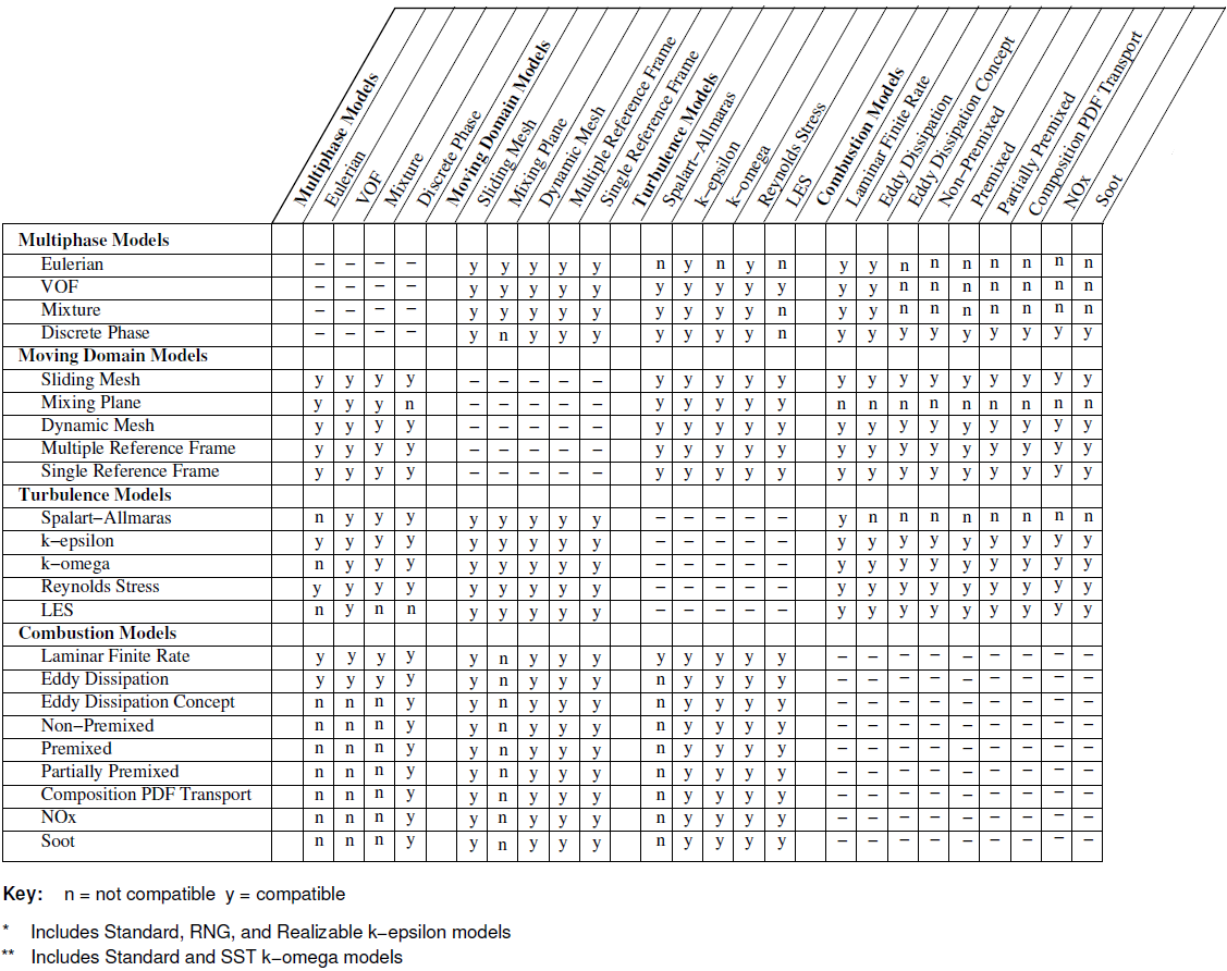
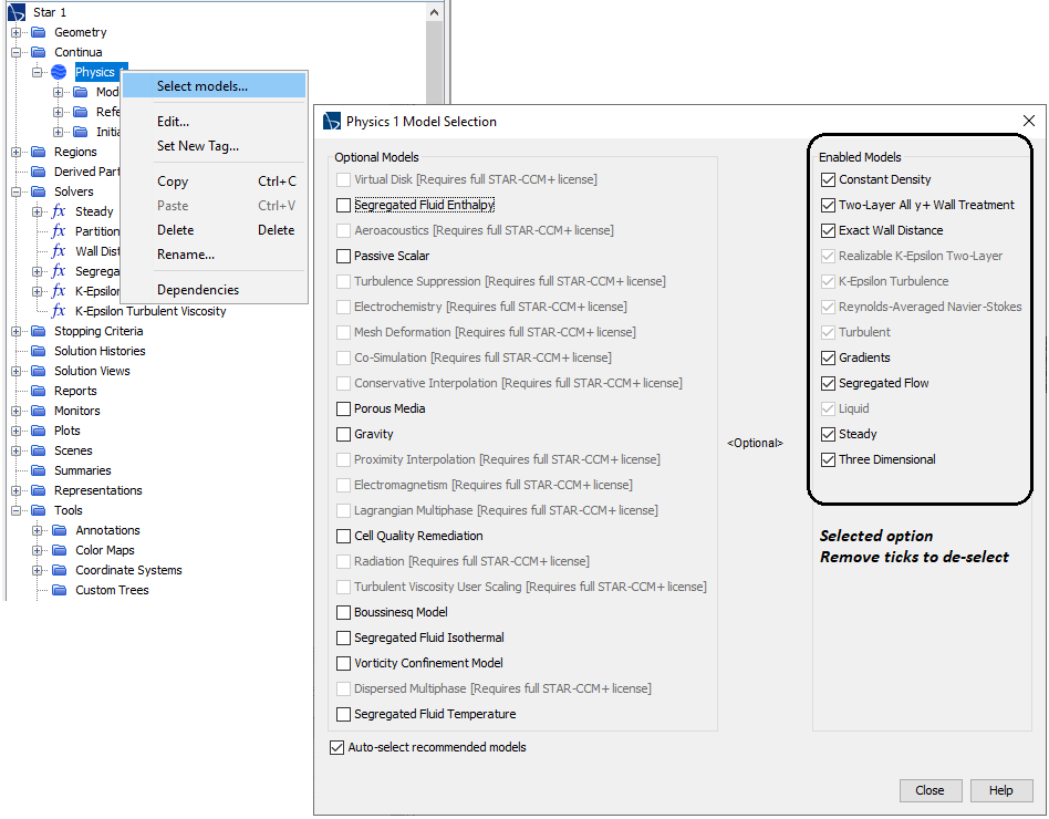
Compatibility of several ANSYS FLUENT model with underlying physics and turbulence model are tabulate below (reference ANSYS FLUENT User's Guide)
Default Settings of Solvers
The GUI of solvers at start-up comprises of layout (of various windows), default value of material properties, number of contour bands, number of decimal places, a specific license configuration, parallel configuration (such as n-2 cores of the machine), working directory, solution backup interval, units, default view of graphics windows... Most of the programs have a text file stored which can be edited to change the default behaviour.
STAR-CCM+ uses a folder C:\Users \UserName \AppData \Local \CD-adapco \STAR-CCM+ <version> - deleting this folder shall reset both the GUI and other custom settings in Simcenter STAR-CCM+. Sometimes, GUI can be used to reset the GUI such as in STAR-CCM+ use: Tools > Reset Options > Window Layouts. To reset the GUI settings using a command prompt, type "starccm+.exe -reset".
FLUENT auto executes the .fluent file in the "home directory" of Linux users, C:\ directory on Windows machines. A .fluent file can contain any number of scheme file names to load. Unless full path is specified for each scheme file in .fluent file, FLUENT tries to locate the scheme files from the working directory. Some users create a SCHEME journal file as per their needs and manually run it in TUI: file/read-journal after FLUENT session has opened, or using typically just 5 button clicks in the GUI. For recent versions, the default settings are stored as JSON (nested dictionary) file in ~/.fluentconf/version/preferences file.
Not all options in File > Preferences... are available as per the 'preferences' file. For example, GraphicsDefaultManualFaceColor can be used to set the face colour to create mesh views though Graphics > Mesh.To change default values in ANSYS CFD-Post, for example changing the Default Number of Contours from 11 to 16, or changing the Default Range choice from Global to Local: the file <ANSYS Inc>/CFD-Postetc/CFXPostRules.ccl needs to be edited. E.g. %3.0f can be used instead of %10.3e to change as Fixed and 0 decimal place.
Compressibility of Fluids
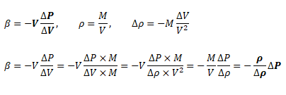
One of the key consideration is the compressible or incompressible behaviour of the fluid. For liquids under lower pressure conditions (except cases such as hydraulics, deep bore drilling in oil exploration...), they can be assumed incompressible without loss of any accuracy. The compressibility chek for liquids need to be decided based on bulk modulus, operating pressures and coefficient of volume expansion.. The later varies between 0.001 ~ 0.010 [K-1]. The bulk modulus is defined as β = -V × ΔP/ΔV where negative sign refers to the fact that volume decreases as pressure increases. Thus, in terms of density, β = -ρ/Δρ × ΔP. β for water is 2.2 [GPa]. Hence, at pressure of 100 [MPa], the change in water density as compared to density at 1 [atm] would be 1000 [kg/m3] × 0.1 [GPa] / 2.2 [GPa] = 45.5 [kg/m3] which is 4.55% of density of water at 1 [atm].
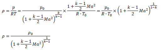
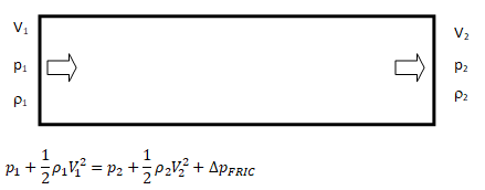
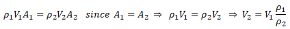
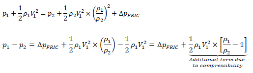
While the change in density of liquids is more pronounced with change in temperature, the situation is different in cases of gases where density is a strong function of both temperature and pressure changes. Note that the density is calculated based on static conditions (static temperature and static pressure) and not on total conditions (total temperature and total pressure). On the other hand, the stagnation conditions are the true measure of pressure energy and internal energy. There are two modes of reduction in stagnation (or total) pressure: the first mode is due to conversion of pressure energy into velocity (kinetic) energy and the second mode is loss of pressure energy due to wall friction and minor losses (sudden expansion and contraction). The general equations to estimate stagnation and static conditions for all values of flow velocities are described below.
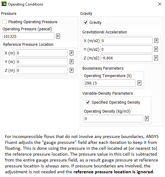
The operating pressure is used to specify the mean pressure in the system. Though it can be adjusted to convert the gauge pressure into absolute pressure. That is, the operating pressure can be set to zero to get the pressure field directly in absolute values. This is the recommended method for cases involving phase change such as simulation of cavitation in pumps. Note that cavitation occurs when local absolute static pressure in the flow field falls below saturation pressure at given temperature. However, once the operating pressure is set to 0 [Pa], the boundary conditions should also be specified in absolute values, e.g. 1,01,325 [Pa] instead of 0 [Pa].
ANSYS FLUENT provides an option of incompressible-ideal-gas available in ANSYS FLUENT makes the density a function of temperature only. This option does not take into account change in density due to variation of pressure and hence should be used when temperature variations are large but pressure variations are small. How to solve isothermal flows with significant variation in pressure? One option is to use Ideal Gas and turn off the energy equation. Thus, temperature shall remain constant and pressure field is anyway solved by momentum equation. Another option is to use an UDF to define density as a function of pressure and constant temperature.
Near atmospheric pressure, and in non-vacuum systems, the continuum theory (called macroscopic in nature) accurately describes the properties of gases when collisions between gas molecules determines the properties of a gas. Under vacuum conditions, gas molecules become so sparse that inter-molecular collisions no longer dominates, and the collisions between gas molecules and the chamber walls become determining factor affecting the gas properties. Air which contains 78% nitrogen, the Knudsen number based on mean free path of nitrogen at 1,000 [Pa] pressure is approximately 0.00034 [m] / 0.025 [m] = 0.014. Thus, the continuum hypothesis shall not hold true for air if pressure reduces close to 1,000 [Pa] which is approximately 100 times less than atmospheric pressure.
The solver-setting process encompasses following aspects of numerical solutions.
- Discretization scheme for momentum, pressure, energy and turbulence parameters: The PRESTO (Pressure Staggering Option) is recommended for pressure because in flows with high swirl numbers.
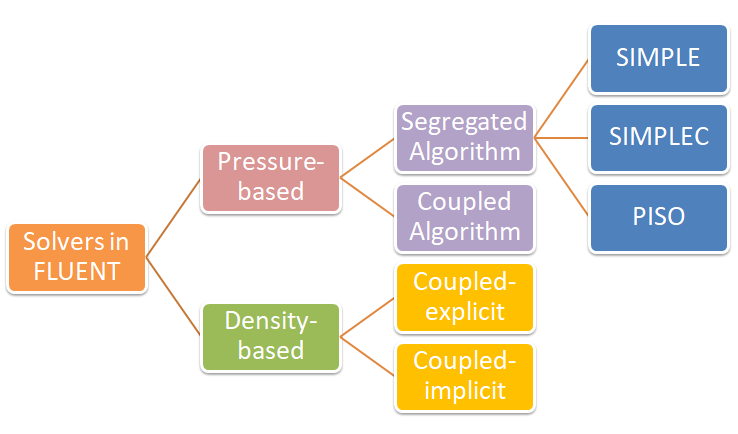
- PV-Coupling such as SIMPLE, SIMPLEC, SIMPLER, PISO
- Gradient schemes: Green-Gauss node based or Green-Gauss cell-based.
On irregular (skewed and distorted) unstructured meshes, the accuracy of the least-squares gradient method is comparable to that of the node-based gradient (and both are much more superior compared to the cell-based gradient).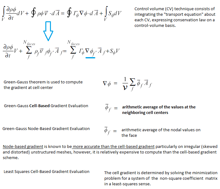
- Conservation target and residual levels for convergence criteria. In addition to the "residual norm", it is strongly recommended to set "mass-conservation" or "energy-conservation" as convergence check.
- Fluid time-scales
- Solid time-scales (in case of conjugate heat transfer or pure conduction problems). The recommended practice is to have solid time-scale set to an order of magnitude (10 times) higher than fluid time-scale.
- One should ensure that the solution is mesh-independent and use mesh adaption to modify the mesh or create additional meshes for the mesh-independence study. A mesh-sensitive result confirms presence of "False Diffusion".
- The node-based averaging scheme is known to be more accurate than the default cell-based scheme for unstructured meshes, most notably for triangular and tetrahedral meshes.
- Note that for coupled solvers which solves pseudo-transient equations even for steady state problems (such as CFX), relaxation factors are not required to be set. The solver applies a false time step as the convergence process is iterated towards final solution.
- QUICK or Geo-Reconstruct scheme for the volume fraction in FLUENT
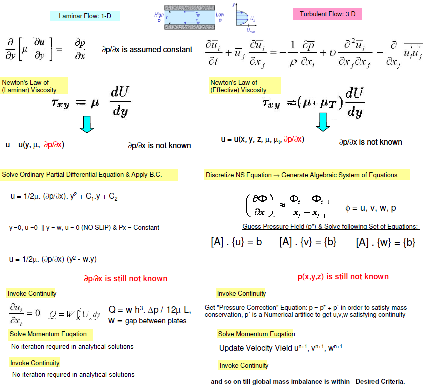
SIMPLE Algorithm: Analogy between analytical solution and numerical simulation
Differences between collocated (non-staggered) and staggered grid layout
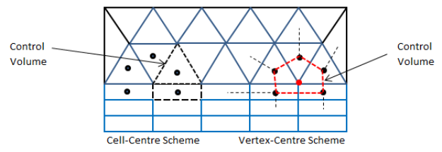
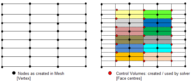
- For collocated solvers (such as ANSYS CFX), control volumes are identical for all transport equations, continuity as well as momentum.
- CFX is a node-based solver and constructs control volumes around the nodes from element sectors, thus the number of control volumes is equal to the number of nodes and not the number of elements. The input of CFX may be tetrahedron, prism and hexhedron in physical form, the solver internally generates a polyhedral mesh. In a cell centered code, such as FLUENT or STAR-CD / STAR-CCM+, number of elements are the same as the number of control volumes (as the control volumes are same as physical elements) so these are often used interchangeably.
- Node-based Solvers: All field (or unknown or solution) variables as well as fluid properties are stored at the nodes (the vertices on the mesh).
- The distinction between collocated and staggered approach is nicely explained in section 4.6 by S. V. Patankar in his book "Numerical Heat Transfer and Fluid Flow" and section 7.2 in the book Computational Methods for Fluid Dynamics by J. H. Ferziger and M. Peric.
- For staggered (cell-based) solvers like ANSYS FLUENT, values of scalar field variables as well as material properties are stored as cell centres.
- Due to the difference in the way field variables are stored, the simulation with same mesh, material properties and boundary conditions, the y+ value reported in ANSYS CFX will be approximately twice that reported in FLUENT.
Compress Solution Files
The file size of set-up files generated during CFD simulations is relatively large depending upon the number of cells and physics solved. Large files take time to upload/download and even compression-decompression is time consuming. However, compression is only feasible option to minimize issues related to data transfer. On Windows: while creating/splitting zip files using 7zip, there is option to choose the number of threads for parallel processing which can be used to ZIP the file or folder quickly. However, UNZIP operation inherently runs in serial mode. In Linux: "tar -cvzf zippedFolder.tar.gz f1.pdf f2.docx f3.msh dirReports" can be used to compress/tar files and folders together. However, it works in serial mode only. Also, a double precision solver shall produce result files significantly bigger than single precision solver.Single Precision vs. Double Precision
If you try to calculate 21024 in LibreOffice Calc, you will get #Num! which is an indication that the number cannot be stored. 2^1023.99999999999 = 1.79769313485112E+308, if you try 2^1023.999999999994 then the values in the formula shall get changed to 2^1023.99999999999 and calculated value shall get changed to 1.79769313485481E+308. If you try to increase the number of significant digits, maximum you can go up to 1.79769313485481000000E+308. Why is it so? Why LibreOffice Calc is not able to calculate 2^1024? Why it is not able to store more than 14 digits after decimal place? It shall store 9.99999999999999 and any additional digit after decimal shall get truncated or rounded-off. Attempt to type 9.999999999999991 gets truncated to 9.99999999999999, attempt to type 9.999999999999992 gets rounded-off to 10. All these computations are being tried out on a Laptop with 64-bit AMD processor and Ubuntu OS.Few basics before learning how computers store numbers. Bit = 0 or 1, Nibble = 4 bits, Byte = 8 bits, 1 Word = 4 bytes, usigned = positive numbers, left most bit of a byte is called most significant bit and the right most as least significant bit, halfword or double byte contains 16 bits. MSB (Most Significant Bit) is used to indicate if the number is negative or positive: MSB = '1' means '-' and MSB = '0' means '+'. Each character (in ASCII table) requires 8 bits (1 byte) of storage. However, the number 1.23E-4 does not require 7 characters x 1 byte/character = 7 bytes or 28 bits to get stored digitally. So how does a decimal number gets stored digitally?
The paper "On floating point precision in computational fluid dynamics using OpenFOAM" by F. Brogi et. al. gives a real life example of impact of single precision solver on accuracy, convergence and computation time. Other references: amd.com/ ... /single-precision-vs-double-precision-main-differences.html and mathworks.com/ ... /floating-point-numbers.html
| Description | Single-Precision | Double-Precision |
| Overview: x= (−1)s.(1+f).2e | Uses 32 bits of memory to represent a numerical value, with one of the bits representing the sign of mantissa | Uses 64 bits of memory to represent a numerical value, with one of the bits representing the sign of mantissa |
| Base, s: | 0 for positive number, 1 for negative number | |
| Biased exponent, e: | 8 bits used for exponent | 11 bits used for exponent |
| *Fraction or Mantissa, f: precision bits of numbers | Uses 23 bits for mantissa (to represent fractional part) | Uses 52 bits for mantissa (to represent fractional part) |
| Definition in programming languages | Float, Single, int32, uint32 | Real, Double, int64, uint64 |
| Minimum** | -2127 ≈ -3.4E-038 | -21023 ≈ -2.225e-308 |
| Maximum** | 3.40E-38 | 1.798E+308 |
Tips: In case the solver set-up is too big to get accommodated in available RAM size, try switching to single precision version of the solver, at least for the initial run till a machine with higher RAM can be arranged. The file size with single precision version shall be approx. half of that of double precision version. As per Microsoft "Data type summary":
| Data type | Storage size | Range |
| Boolean | 2 bytes | True or False |
| Byte | 1 byte | 0 to 255 |
| Decimal | 14 bytes | +/- 79,228,162,514,264,337,593,543,950,335 with no decimal point +/- 7.9228162514264337593543950335 with 28 places to the right of the decimal. Smallest non-zero number is +/- 0.0000000000000000000000000001 |
| Double* | 8 bytes | -1.79769313486231E308 to -4.94065645841247E-324 for negative values. 4.94065645841247E-324 to 1.79769313486232E308 for positive values |
| Integer | 2 bytes | -32,768 to 32,767 |
| Long integer on 32-bit systems | 4 bytes | -2,147,483,648 to 2,147,483,647 |
| Long integer on 64-bit systems | 8 bytes | -9,223,372,036,854,775,808 to 9,223,372,036,854,775,807 |
| Single* | 4 bytes | -3.402823E38 to -1.401298E-45 for negative values. 1.401298E-45 to 3.402823E38 for positive values |
Mark Bad Cells
Separating cells by Mark (Adaptation Register) /mesh/modify-zones/slit-face-zone 3 5 (): slit the faces of wall zones 3 and 5, either delete or deactivate the separated cell zone.To mark and display bad cells, use "Cell Register" from model structure tree and then select 'Mesh' under "Field Value of" drop-down. This option is available only when fields are initialized.
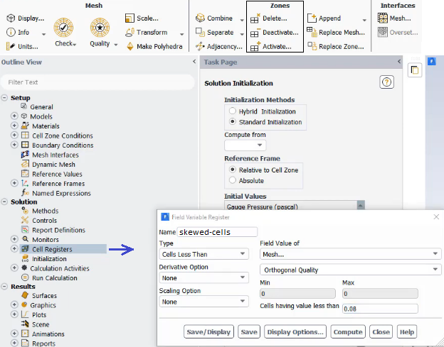
Alternatively, use Adapt Iso-value Mesh Select the property you want to adapt (e.g. Skewness or Orthogonal Quality in this case) Click 'Compute" to get the minimum and maximum value of the property in the domain Set the minimum and maximum bounds to select cells between these bounds. For example, you can set skewness with min 0.95 and max 1.0 to select all cells with a skewness bigger than 0.90 Click Adapt to remesh them.
Solver Setting: Physics
The flow regime and classification of laminar, transition and turbulent zones are unique to every flow. One of the most widely used flow condition is flow over a cylinder in cross flow. The following summary is an interesting description of how the flow evolve:- Re ≤ 5, flow is laminar throughout and no vortices are present downstream of the body.
- 5 < Re < 40, a vortex pair can be observed in the wake region though flow is still laminar in the boundary layer.
- 40 ≤ Re ≤ 200, a von Karman vortex street is formed as where pairs of counter-rotating vortices are shed downstream of the body. The vortex shedding frequency is given by a non-dimensional Strouhal number: St = f × D / U.
- 200 ≤ Re ≤ 300, the flow behind a cylinder undergoes transition to a turbulent wake.
- 300 ≤ Re ≤ 3×10⁵, the sub-critical Reynolds number regime wake is turbulent while the boundary layer is still laminar.
- Re > 3×10⁵, a transition from laminar to turbulent boundary layer separation occurs.
Solver Setting for Transient Simulation: CFL Number
Many a time, it is difficult to decide whether the physical behaviour of system is transient, quasi-transient and steady state. Following example can be used to check if solution should be solved as steady state problem or a transient simulation.

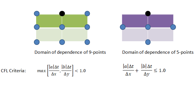
In an explicit Eulerian method, the Courant number cannot be > 1 otherwise it will lead a condition where information is propagating through more than one grid cell at each time step. This is explained in the physical domain of dependence and numerical domain of dependence in following diagram. For a stable solution, numerical domain of dependence must cover the physical (real) domain of dependence.
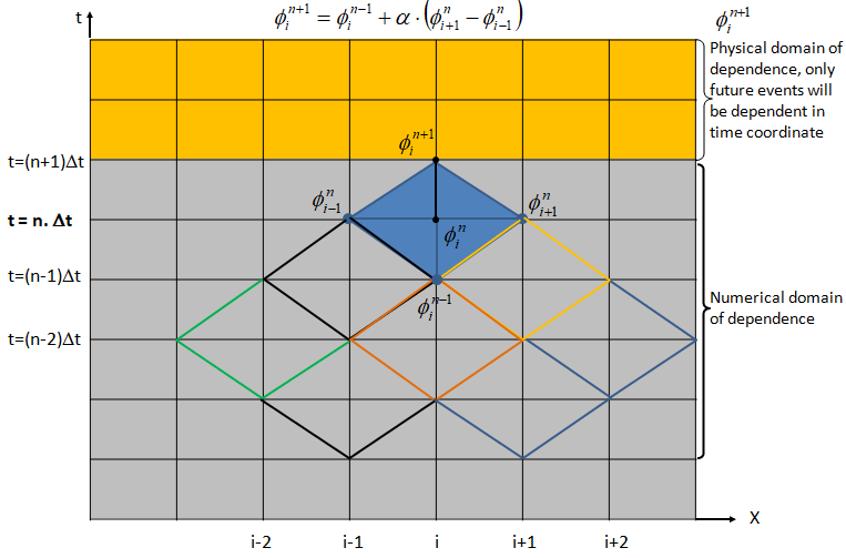
Thus, Courant number can be reduced either by reducing the time step or by increasing the mesh size (i.e. coarsening of the mesh). The later option may appear counter-intuitive though mathematically that remains a fact. It is difficult for most of the simulation engineers to believe the fact that coarsening the mesh help them achieve a better convergence.
- The CFL number scales the time-step sizes that are used for the time-marching scheme of the flow solver.
- A higher value leads to faster convergence but can lead to divergence and unstable simulations. The (stiff) CFL condition can be relaxed or softened by using implicit Euler such as Crank–Nicolson which is unconditionally stable.
- The inverse of this is also true where choosing a smaller value in an unstable simulation improves convergence.
- ANSYS FLUENT uses implicit (first order and second order) formulation for pressure-based solver. As per the user guide: "It is best to select the Coupled pressure-velocity coupling scheme if you are using large time steps to solve your transient flow, or if you have a poor quality mesh."
- In general, the solution at the end of (inner iterations in) current time-step is used as initial value for iterations at next time-step. ANSYS FLUENT provides option to extrapolate the solution variable values for the next time step using a Taylor series expansion. This can improve the convergence of the transient calculations by enabling and the absolute residual levels are lowered during inner iterations.
To verify that your choice for time-step was proper, check contours of the Courant number within the domain. In FLUENT, select Cell Courant Number under Velocity... For a stable and accurate calculation, the Courant number should not exceed a value of 20-40 in most sensitive transient regions of the domain.
Note that CFX reports two types of Courant number: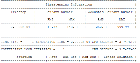
Material Properties
Sometime underlying physics and type of solver chosen governs the material definition. For example, a density based solver requires density to be function of pressure and temperature. Similarly, simulation of Joule-Thomson phenomena (cooling effect due to throttling) requires material properties to be modeled as real-gas. An ideal gas will never cause this effect. The simulation related to steams required careful understanding of state of steam: wet-steam vs. dry steam. An incompressible flow may required only density and viscosity of a fluid whereas phase change and/or reacting mixture phenomena will require definition of reference enthalpy and entropy.Similarly, air can be treated as 4 different ways depending upon application such as:
| Air for common applications | Air in HVAC and Psychrometrics | Air in Hydrocarbon Fuel Combustion | Air in Pneumatic and High Pressure applications |
| Ideal gas with molecular weight = 28.96 [g/mole] | Mixture of gases: Dry air + Water vapour | Mixture of gases: Oxygen, Nitrogen, Water Vapour, Argon | Real Gas with behaviour different from ideal gases |
In some applications such as fans, there are significant reduction in pressure values (such as trailing edge and flow separation regions) as well as significant increase in pressure values (near leading edge). Hence, flow simulations dealing with gas and turbo-machine should use ideal gas law as final settings. Constant density can be used initially to get a convergence. The option of incompressible-ideal-gas available in ANSYS FLUENT makes the density a function of temperature only. This option also does not take into account change in density due to variation of pressure near the blade tip and separation regions.
To get a better accuracy, temperature dependent properties should be used. Some correlations available for gases are tabulated below. The Sutherland coefficients for some common gases are as follows. μ = μ0 * (273+C)/(T+C)*(T/273)1.5 where C is Sutherland coefficient in [K], T is fluid temperature in [K] and μ is viscosity in [Pa.s]. Reference: Handbook of Hydraulic Resistance by I. E. Idelchik.
| Fluid | μ0 [Pa.s] | C [K] |
| Air | 17.12 | 111 |
| N2 | 16.60 | 104 |
| O2 | 19.20 | 125 |
| CO2 | 13.80 | 254 |
| H2O-g | 8.93 | 961 |
| H2 | 8.40 | 71 |
The variation in dynamic viscosity of air in the temperature range 0 to 100 [°C] is of the order of 25% which is a significant amount if the wall friction contributes more to the pressure drop in the system. Similarly, a 5% reduction in local pressure shall cause 5% reduction in density and hence the velocity or volume flow rate has to increase by 5% to ensure the mass balance.
Specific Heat Capacity - Reference: B. G. Kyle, Chemical and Process Thermodynamics - Cp [kJ/kmol-K] ≡ [J/mol-K] = a + b.T + c.T2 + d.T3 where T is in [K]. For air, the coefficients are: a = 28.11 [kJ/kmol-K], b = 1.967E-03 [kJ/kmol-K2], c = 4.802E-06 [kJ/kmol-K3], d = -1.966E-09 [kJ/kmol-K4]. Taking molecular weight of air to be 28.96 [kg/kmol], the coefficients to calculate Cp in [J/kg-K] are: a = 970.65 [J/kg-K], b = 0.06792 [J/kg-K2], c = 1658E-04 [J/kg-K3], d = -6.788E-08 [J/kg-K4]. As you can notice, there is ~1% variation in specific heat capacity of air over the range of 100 [°C] and hence it can be assumed a constant value in calculations and simulations. Also note that for steady state simulations, the specific heat capacity and even density is not needed for solids. This can be inferred from the conduction equation for steady state conditions where only thermal conductivity appears as coefficient.
Thermal Conductivity - Reference: B. G. Kyle, Chemical and Process Thermodynamics - k [W/m-K] = a + b.T + c.T2 + d.T3 where T is in [K]. a = -3.933E-04 [W/m-K], b = 1.018E-04 [W/m-K2], c = -4.857E-08 [W/m-K3], d = 1.521E-11 [W/m-K4]. There is 25% increase in thermal conductivity or air in the temperature range 15 ~ 100 [°C] and hence a constant thermal conductivity may yield lower heat transfer rate.
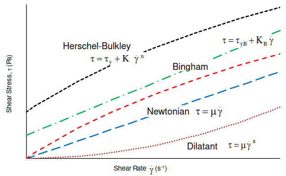
Non-Newtonian Fluids: Most of the fluids behave such that shear stress is linear function of strain rate with zero initial threshold value of shear stress. However, there are some material where shear stress is non-linear function of strain rate with non-zero initial threshold value of shear stress (yield point) before which flow cannot start. Various type of such material also known as Bingham plastic and Herschel-Bulkley are described below.
Use material properties as tabulated data function of p and T: In STAR-CCM+ use "Physics Simulation > Materials > Setting Material Properties Methods > Using Table (T, P)". In ANSYS FLUENT, File > Table File Manager... > Read... In ANSYS FLUENT V24, an expression for density cannot be defined in terms of both the Absolute Pressure and Static Temperature. Error reported is: "Density expression cannot be a function of both Absolute Pressure and Static Temperature".

import numpy as np
def bilinear_interpolation(grid, x_var, y_var, x, y):
  '''
  Args:
    grid (np.array): A 2D array representing the data (dependent variable)
    x_var (np.array): 1D array of x - independent variable 1
    y_var (np.array): 1D array of y - independent variable 2
    x (float): The value of x to interpolate at
    y (float): The value of y to interpolate at
  Returns: The interpolated value at (x, y).
  '''
  # Find the grid indices surrounding the point
  x_idx = np.searchsorted(x_var, x, side="right") - 1
  y_idx = np.searchsorted(y_var, y, side="right") - 1

  #Check if interpolation points falls inside data grid
  if x_idx<0 or y_idx<0 or x_idx >= len(x_var)-1 or y_idx >= len(y_var)-1:
    return np.nan

  x1, x2 = x_var[x_idx], x_var[x_idx + 1]
  y1, y2 = y_var[y_idx], y_var[y_idx + 1]

  # Get the values of the four corners
  q11 = grid[y_idx,     x_idx]
  q12 = grid[y_idx,     x_idx + 1]
  q21 = grid[y_idx + 1, x_idx]
  q22 = grid[y_idx + 1, x_idx + 1]

  # Check for division by 0, perform the interpolation
  if x2 == x1 or y2 == y1:
    return q11
  x_weight = (x - x1) / (x2 - x1)
  y_weight = (y - y1) / (y2 - y1)

  interpolated_value = (
    q11 * (1 - x_weight) * (1 - y_weight) +
    q12 *      x_weight  * (1 - y_weight) +
    q21 * (1 - x_weight) * y_weight       +
    q22 *      x_weight  * y_weight
  )
  return interpolated_value

grid = np.array([[1, 2, 4], [4, 5, 10], [7, 8, 12]])
x_c = np.array([0, 5, 9])
y_c = np.array([0, 2, 4])
x_interp = 2.5
y_interp = 1.0
interp_value = bilinear_interpolation(grid, x_c, y_c, x_interp, y_interp)
print(f"Interpolated value at ({x_interp}, {y_interp}): {interp_value}")
Mass Fraction to Volume (or Mole) Fraction: ensure that the sum of mass fractions add to 1.0, no checks are performed in case they do not. Typically method to check the correctness of following method is to specify same value of mass fractions (0.5 or 50%) and density for both phases, the calculated volume fractions should be equal to 0.50 (50%) for both phases.
| First phase mass fraction [%] and density [kg/m3] | β1: | % | ρ1: | |
| Second phase mass fraction [%] and density [kg/m3] | β2: | % | ρ2: | |
| Volume fraction of the two phases | α1: | % | α2: | % |
Formula to convert mass fraction to volume fraction and vice versa:
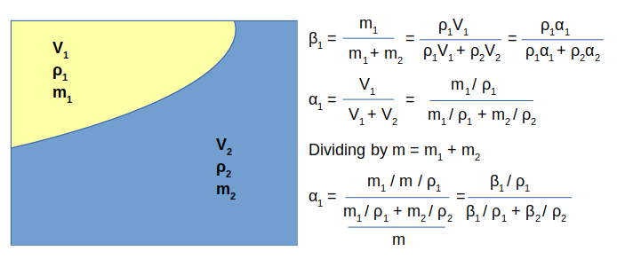
Volume Fraction to Mass Fraction: ensure that the sum of volume fractions add to 1.0, no checks are performed in case they do not.
| First phase volume fraction [%] and density [kg/m3] | α1: | % | ρ1: | |
| Second phase mass fraction [%] and density [kg/m3] | α2: | % | ρ2: | |
| Mass fraction of the two phases | β1: | % | β2: | % |
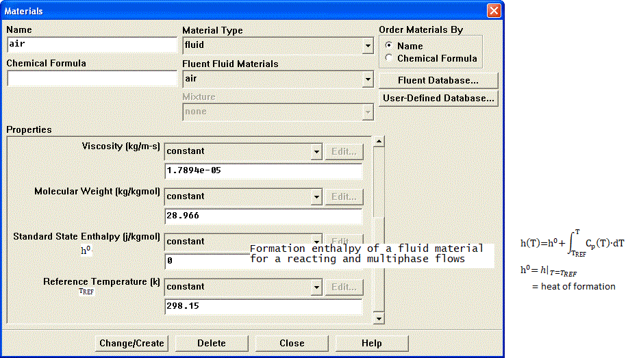
The value of ΔH0 will be negative if the process is endothermic (that is the reaction for material formation requires external heat energy) or positive if the process is exothermic (if heat is released during formation or reaction).
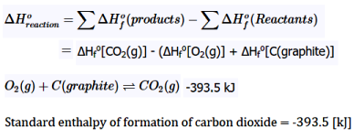
In situations with phase change such as forced convection subcooled nucleate boiling, the standard state enthalpies of vapor and liquid phase are set such that their difference equals to latent heat of vapourization = 2.992E+07 [J/kmole]. The unit of standard state enthalpy is [kJ/kmol] and usually the latent heat value is available in [kJ/kg]. The latest heat value in [kJ/mole] should be multiplied by molecular wight of the liquid. For correct specification of latent heat, the reference temperature should be set to 298.15 [K] or 25 [°C]. Note that it is a positive value (in case of boiling simulation) as compared to standard state enthalpies of species such as CO2 and CH4 (which are negative by sign convection) used in species transport and combustion modeling.
In phase change phenomena (evaporation and/or condensation), the difference between actual temperature of the phase and saturation conditions are described as degree of sub-cooling (liquid) and degree of super-heating (gas). If the inlet temperature of liquid is T = 350 [K] and the saturation temperature TSAT = 373 [K], liquid state is terms as sub-cooled and with the degree of sub-cooling = 373 - 350 = 23 [K]. In a nucleate boiling, when the wall temperature rises above the liquid saturation temperature, steam bubbles will get formed and migrate away from the wall. Since the bulk flow (liquid far away from the wall) is sub-cooled, these bubbles condense near the center of the pipe.
Wet Steam: The steam with droplets of water is known as wet steam and it characterized by dryness fraction. Most of the boilers do not generate dry steam as steam bubbles breaking through the heated surface will pull tiny water droplets along with it. In general, when a substance exists partly as liquid and partly as vapour (gas) phase, its quality is defined as the ratio of the mass of vapor to the total mass. On the hand, mass fraction of the condensed phase is known as wetness factor.
Dry Steam: Saturated or superheated steam are known as dry steam.
For water, the triple point T = 0.01 [°C] and P = 0.6113 [kPa], is selected as the reference state where the internal energy, enthalpy and entropy of saturated liquid are assigned a zero value. Similarly, saturated refrigerant R-134a is specified enthalpy of 0 [J/kg] at temperature -40 [°C] and pressure of 51.25 [kPa]. Thus, standard state enthalpy of liquid water is 0 and reference temperature is 273.15 [K]. The standard state enthalpy of steam is heat of vaporization at T = 0.01 [°C] and P = 0.6113 [kPa] and equals 2501 [kJ/kg]. The molecular weight of water is 18.0153 [kg/kmole] and hence the standard state enthalpy of steam is (2501 × 18.0153) [kJ/kmole]. The saturation pressure of water as per ASHRAE: p(T in [K]) in [Pa] = exp[c1 / T + c2 + c3 * T + c4 * T2 + c5 * T3 + c6 * Ln(T)] where c1 = -5800.22, c2 = +1.3914993E+00, c3 = -4.8640239E−02, c4 = +4.1764768E−05, c5 = −1.4452093E−08, c6 = +6.54597.Porous Domains
Flow geometry such as heat exchangers with closely spaced fins, honeycomb flow passages in a catalytic converters, screens or perforated plates used as protection cover at the from of a tractor engine ... are too complicated to model as it is. They are simplified with equivalent performance characteristic, knowns as Δp-Q curve. These curves are either generated using empirical correlations from textbooks or using a CFD simulation for small, periodic / symmetric flow arrangement. The simplified computational domain is known as "porous zone" in case it is represented as a 3D volume or pressure or porous jump in case it is represented as a plane of zero thickness. In a similar fashion, the performance data of a fan can be specified including the swirl component.All the porous media formulation take the form: Δp = -L × (A.v + B.v2) where v is the 'superficial' flow velocity and negative sign refers to the fact that pressure decreases along the flow direction. The 'superficial velocity' is calculated assuming there is no blockage of the flow. L is the thickness of the porous domain in the direction of the flow. Here, A and B are coefficients of viscous and inertial resistances.
In FLUENT, the equation used is: Δp/L = -(μ/α.v + C2.ρ/2.v2) where α is known as 'permeability' and μ is the dynamic viscosity of fluid flowing through the porous domain. This (permeability) is a measure of flow resistance and has unit of [m2]. Other unit of measurement is the darcy [1 darcy = 0.987 μm2], named after the French scientist who discovered the phenomenon.
STAR-CCM+ uses the expression Δp/L = -(Pv.v + Pi.v2) for a porous domain.
The pressure drop is usually specified as Δp = ζ/2·ρ·v2 where ζ is 'equivalent loss coefficient' and is dimensionless. Darcy expressed the pressure gradient in the porous media as v = -[K/μ]·dP/dL where 'K' is the permeability and 'v' is the superficial velocity or the apparent velocity determined by dividing the flow rate by the cross-sectional area across which fluid is flowing.Steps to find out viscous and inertial resistances:
- Calculate the pressure drop vs. flow velocity data [Δp-v] from empirical correlations or wind-tunnel test or simplified CFD simulations.
- Divide the pressure drop value with thickness of the porous domain. Let's name it as [Δp'-v curve].
- Calculate the quadratic polynomial curve fit coefficients [A, B] from the curve Δp'-v. Ensure that the intercept to the y-axis is zero.
- In STAR-CCM+ these coefficients 'A' and 'B' can be directly used as Pv and Pi which are viscous and inertial resistance coefficients respectively.
- Divide 'A' by dynamics viscosity of the fluid to get inverse of permeability that is 1/α [m-2] to be used in ANSYS FLUENT as "viscous resistance coefficient" [m-1].
- Divide 'B' by [0.5ρ] where ρ is the density of fluid, to get C2 to be used in ANSYS FLUENT as "inertial resistance coefficient".
- The method needs to be repeated for the other 3 directions. If the flow is primarily one-directional, the resistances in other two directions need to be set to a very high value, typically 3 order of magnitude higher.
In case porous domain is not aligned to any coordinate direction, the direction of unit vector along the flow and across the flow directions can be estimated from following Javascript program. Note that empty field is considered as 0.0. There is no check if a text value is specified in the input fields and the calculator will result in an error.
| First point - X1: | |
| First point - Y1: | |
| First point - Z1: | |
| Second point - X2: | |
| Second point - Y2: | |
| Second point - Z2: | |
Temperature Drop across a Porous Domain
If flow through the porous domain is assumed (a) incompressible, one-dimension, steady state and (b) pressure drop varies linearly with the flow direction x: 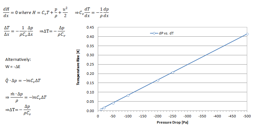
Named Expressions
The newer versions of program FLUENT and STAR-CCM+ have option to use named expression and field functions for customized boundary conditions. This eliminate need to write an UDF (User Defined Function). For example, following 5 expressions can be used to define inlet mass flow rate (kg/s) as function of static pressure (Pa) at outlet where mass flow rate is a parabolic function of pressure mdot [kg/s] = C0 [kg/s] + C1 [m.s] × pr + C2 [m^2 s^3 kg^-1] × pr2. Here pr = MassFlowAve(StaticPressure, ['Outlet']).Radiation Modeling
The selection of Radiation Model is based on optical thickness = a x L where L is typical length scale and a absorption coefficient. OpenFOAM provides three radiation models: P1 model, fvDOM (finite volume discrete ordinates model) and viewFactor model.If a x L >> 1 then P1 model. If a × L < 1, use of fvDOM is recommended. Since fvDOM also captures the large optical length scales, it is the most accurate model though it is computationally more intensive since it solves the transport equation for each direction. fvDOM can handle non gray surfaces (dependence of radiation on the the solid angle is included). viewFactor method is recommended if non-participating mediums are present (spacecraft, solar radiation).
ANSYS FLUENT offer following radiation models: Rosseland, P1, Discrete Transfer (DTRM), Surface to Surface (S2S) and Discrete Ordinates (DO). P1, DO, or Rosseland radiation model in ANSYS FLUENT can be used in cases of participating media (where the fluid participated in radiative heat transfer, example exhaust smoke). It is required to define both the absorption and scattering coefficients of the fluid. When using the Rosseland model or the P1 model, the refractive index for the fluid material only should be defined.
TUI for Radiation Setting: /define/models/radiation discrete-ordinate? , , , , where comma is used to accept default values. The 4 inputs needed are (1)Number of θ divisions (2)Number of φ division (3)Number of θ pixels and (4)Number of φ pixels.
The TUI to define emissivities for the walls is: /define/b-c/wall <wall name> , , , , , , , , , 0.40 , , , , where the emissivity is 0.40 and comma is used to accept default values. This TUI command sets the wall as OPAQUE. Also note that the TUI operation does not accept multiple wall zones and hence the setting has to be provided using a loop on multiple face zones of type wall.Solid Cell Zones Conditions for the DO Model: With the DO model, you can specify whether or not you want to solve for radiation in each cell zone in the domain. By default, the DO equations are solved in all fluid zones, but not in any solid zones. If you want to model semi-transparent media, for example, you can enable radiation in the solid zone(s). To do so, enable the Participates In Radiation option in the Solid dialogue box
Initial Condition
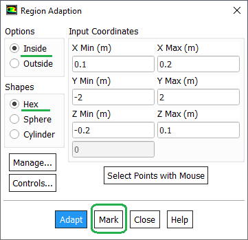
The field variables (u, v, w, p, T, k , ε...) need to be specified certain starting value. It can all be set to 'ZERO' in their respective units or some other physically realistic values. In CFD simulation process, it is called 'initialization' which can be domain (volume specific) or global (applicable to entire computational nodes). For steady-state simulation, the initial condition is a 'wise guess' of the converged steady-state solution. In transient simulations, the initial condition provides the (actual) spatial distribution at t = 0 and hence temporal starting point for the simulation. Thus, for transient simulations, the intermediate result will be strongly influenced the initial condition.In case of multi-phase flow, an initial distribution of volume fraction of the constituents is important. The method to set initial conditions in ANSYS FLUENT is called patching which requires regions to be marked as shown below. In OpenFOAM setFields (requires setFieldsDict) utility is used to initialize field variables in various zones.
Volumetric Heat Sources
ANSYS FLUENT expects heat sources in terms of heat density that is [W/m3] whereas STAR-CCM+ can take directly the heat generation rate [W] for a given volume. In order to check that the total applied heat generated rate is equal to the expected value, initialize the flow field and then calculate heat transfer rate from "Reports -> Fluxes" option. ANSYS FLUENT shall print the total "User Source" that is the total heat generation rate defined by all defined volumetric heat sources.A sample SCHEME script to apply volumetric heat source of 500 [W/m3] to a zone named htr-ss and material defined as steel is as follows: define b-c solid htr-ss yes steel y 1 y 500 n no n 0 n 0 n 0 n 0 n 0 n 0 n no n. The energy should be turned ON and material name should be present before this script is run in TUI. This script is not applicable for rotating reference frames.
Many times, material properties and volumetric heat source are function of pressure and temperature. They might be available in tabular format and a curve fit may not be possible to get a good fit. A user code in STAR-CCM+ is available at "community.sw.siemens.com/.../User-Coding-for-2-dimensional-T-p-Table-interpolation-Linux-OS" which can be adapted for ANSYS FLUENT as well.Set Solution Limits
In ANSYS FLUENT, limiting values for pressure, static temperature, and turbulence quantities can be set to keep the absolute pressure or the static temperature from becoming 0, negative, or excessively large during the calculation. However, there are no static temperature and absolute pressure solution limits for incompressible flows such as those with constant density gases.Define Monitor Points
It is not known in advance how many iterations a particular set-up would require to get fully converged. Using a default high number of iterations say 5000 iterations may end in unnecessary use of computational power. It is strongly advised to use a monitor point such as inlet pressure (when mass flow rate or velocity inlet boundary condition is used) as convergence criteria instead of using only the equation residuals. ANSYS FLUENT has option to specify number of iterations to be used to create a report definition. This can be used in following ways to define convergence criteria.Option-1: Create report definition say rep_200 to compute average inlet static pressure over last 200 iterations. Create another report definition rep_010 to average inlet static pressure over last 10 iterations. Use the third report definition rep_dP = abs(rep_200 - rep_010). The solution can be marked converged if rep_dP ≤ 0.1 [Pa]
Option-2: Create report definition say rep_002 to compute average inlet static pressure over last 2 iterations. Create another report definition rep_001 to get inlet static pressure at last iteration. Use the third report definition dp_frac = abs(rep_002 - rep_001) / rep_001 * 100. The solution can be marked converged if dp_frac ≤ 0.1%
Convergence History
The residuals of continuity, momentum (u, v and w), energy (T), k and ε is used to check the convergence of iterative solution process. Convergence refers to the situation where the calculated value is assumed to tend to correct inversion of equation [A]{x}={b}. To find the cell(s) related to maximum residual, use the TUI: solve/set/expert yes yes no. Here the answers yes, no and not are responses to the questions "Save cell residuals for post-processing? [no]", Keep temporary solver memory from being freed? [no]" and "Allow selection of all applicable discretization schemes? [no]" respectively. To store the residuals in *.dat file, adjust the data file quantities using "File > Data File Quantities" option. This option is available (as on V24R1) in Legacy format only and both cas.gz / dat.gz files should be loaded. The Data File Quantities gets active after script is run in TUI console. If run is already completed, make one iteration so that the specific data fields are created.
Sometimes k (designated as Tke in STAR CCM+) and and ε (referred to as Tdr in STAR CCM+) may be as high as few thousand and the results are reasonable. The scale can be reduced by turning off the normalization for k and ε. Normalization takes the very first iteration's values to normalize all subsequent residuals. When solution already start with a good solution or guess value for k and ε, the first value is already very low, and residuals may not reduce further. It then sometimes can happen that the residual increases instead of decreasing even though the absolute (without normalization) value might still be very low.
In ANSYS FLUENT, the denominator to calculate the scaled residual for the continuity equation of a pressure-based solver is the largest absolute value of the continuity residual in the first 5 iterations. When iteration starts with a good solution, the largest residual of first 5 iterations may be low. Hence in subsequent iterations, significant reduction in order of magnitude of the residuals may not be observed even though the convergence can be deemed to be of good accuracy. Note 'scaling' and 'normalization' of residuals are different and interpretation should be different as well.
Under Relaxation Factors (URF): As per ANSYS documentation and training material, Pressure and Momentum URFs MUST sum to 1.00 and flow stability is best with smaller pressure URF (0.03 is not uncommon).Thin Walls
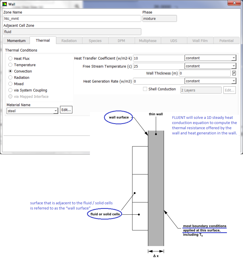
Natural Convection (Buoyancy-driven Flows)
Boussinesq approximation: ρEFF = 1 - β(TWALL - TREF). Here: ρEFF= effective driving density β = coefficient of thermal expansion (equal to 1/T for ideal gas, T in [K]). Boussinesq approximation is only valid for β × (TWALL - TREF) << 1.0 say β × (TWALL - TREF) < 0.10. In other words, the temperature difference should be < 30 [K] for reference temperature of 300 [K].- Use Boussinesq approximation to start the simulation. Specify correct density and expansion factor of the fluid
- Initialize the domain with small velocity say 0.02 or 0.05 [m/s] in the direction opposite to the gravity
- Alternatively, solve a force convection flow with small velocity is expected inlet(s) and then switch on to natural convection mode
- Turn-on radiation once flow and temperature fields have stabilized
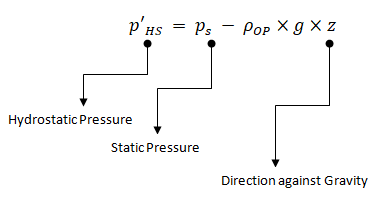
As per FLUENT User's Manual: "The boundary pressures that you input at pressure inlet and outlet boundaries are the redefined pressures as given by equation above. In general you should enter equal pressures, p'HS at the inlet and exit boundaries of your ANSYS FLUENT model if there are no externally-imposed pressure gradients. For example, if you are solving a natural-convection problem with a pressure boundary, it is important to understand that the pressure you are specifying is p'HS. Therefore, you should explicitly specify the operating density rather than use the computed average. The specified value should, however, be representative of the average value. In some cases the specification of an operating density will improve convergence behaviour, rather than the actual results. For such cases use the approximate bulk density value as the operating density and be sure that the value you choose is appropriate for the characteristic temperature in the domain."
Many a time when operating density is not correctly specified, the flow may follow the direction of gravity and no buoyancy effect can be observed. Hence, ad just the operating density calculated at minimum and expected maximum temperature.Refer the document at "innovationspace.ansys.com/.../setting-operating-density-for-natural-convection-cases-when-density-is-modelled-using-ideal-gas-law" to appropriate boundary condition settings.
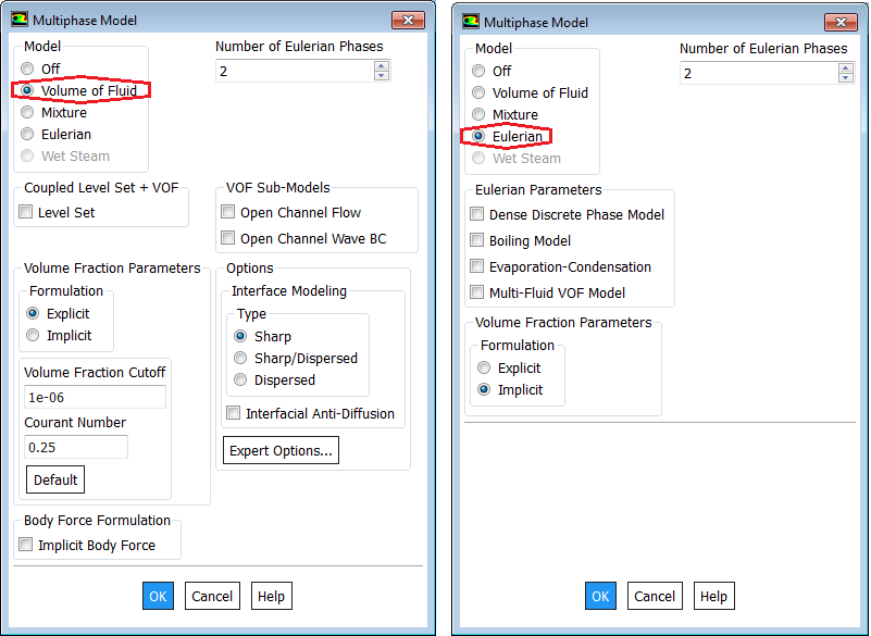
Solver Settings for Multi-Phase Flows
TUI: create the materials before using TUI to set-up multiphase flow in ANSYS FLUENT. Default number of phases = 2. Since air is the default material when a mesh is read, air is assigned primary phase and the second material created is assigned as secondary phase. Let's assume that air and water are the names of the materials.
define models multiphase model eulerian / mixture / vof / none / wetsteam
define phases set-domain-properties phase-domains phase-1 material yes water ()
define phases set-domain-properties phase-domains phase-2 material yes air ()
; Change phase names: specify secondary phase first
define phases set-domain-properties change-phase-names air water

define phases set-domain-properties interaction-domain forces surface-tension sfc-tension-coeff yes 0.072
define phases set-domain-properties interaction-domain forces surface-tension sfc-tension-coeff none

define phases set-domain-properties interaction-domain forces drag yes schiller-naumann yes none ()
define phases set-domain-properties interaction-domain interfacial-area interfacial-area yes ia-symmetric ()
Multi-phase flows have wide applications in process, automotive, power generation and metal industries including phenomena like mixing, particle-laden flows, CSTR - Contunuously Stirred Tanks Reactor, Water Gas Shift Reaction (WGSR), fluidized bed, fuel injection in engines, bubble columns, mixer vessels, Lagrangian Particle Tracking (LPT). Some of the general characteristics and categories of multi-phase flow are described below along with setting parameters in ANSYS FLUENT.
Multiphase flow regimes are typically grouped into five categories: gas-liquid (which are naturally immiscible) flows and (immiscible) liquid-liquid flows, gas-solid flows, liquid-solid flows, three or more phase flows. As can be seen, the immiscibility is a important criteria. In a multi-phase flow, one of the phase is usually continuous and the other phase(s) are dispersed in it. The adjective "Lagrangian" indicates that it relates to the phenomena of tracking a moving points ("fluid particles") - such as tracking a moving vehicle on a road. On the other hand, the adjective "Eulerian" is used to describe correlations between two fixed points in a fixed frame of reference - such as counting the type of vehicles and their speeds while passing through a fixed point on the road.
Gas-liquid flows are further grouped into many categories depending upon the distribution and shape of gas parcels. Three such types are described below.Bubbly Flow: it represents a flow of discrete gaseous or fluid bubbles in a continuous phase.

From FLUENT User Guide V12: "For fluid-fluid flows, each secondary phase is assumed to form droplets or bubbles. This has an impact on how each of the fluids is assigned to a particular phase. For example, in flows where there are unequal amounts of two fluids, the predominant fluid should be modeled as the primary fluid, since the sparser fluid is more likely to form droplets or bubbles."
Some other types of flows are particle-laden flow such as air carrying dust particles, slurry flow where particles are transported in a liquid, hydro-transport which describes densely-distributed solid particles in a continuous liquid such as cement concrete mix. Gas assisted mixing of solid such as fluidized-bed and settling tank where particles tend to sediment near the bottom of the tank forming thick sludge are some other examples of multi-phase flows.
The two dominant method of multi-phase simulations are listed below.
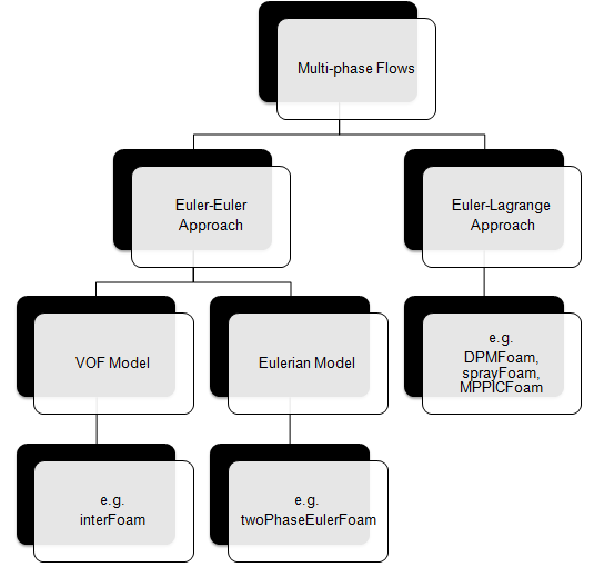
- A phase cannot be occupied by the other phases in space, the concept of "phasic volume fraction" is used and assumed to be continuous functions of space and time. Distribution of phases are plotted by volume fraction whereas in DPM (Euler-Lagrange approach) the distribution of phases are plotted by particle track.
- Globally, the sum of this phasic volume fraction equals to one.
- Conservation equations for each phase are derived as a set of equations having similar structure for all phases, analogous of momentum equations.
- These equations are closed by constitutive relations obtained from empirical information.
Improve convergence behavior of Eulerian Model
Reference: FLUENT User Guide V12- Compute an initial solution before solving the complete Eulerian multiphase model. There are three methods you can use to obtain an initial solution for an Eulerian multiphase calculation:
- Set up and solve the problem using the mixture model (with slip velocities) instead of the Eulerian model. You can then enable the Eulerian model, complete the setup, and continue the calculation with Eulerian Model using the mixture-model solution as a starting point.
- Set up the Eulerian multiphase calculation as usual, but compute the flow for only the primary phase. To do this, deselect Volume Fraction in the Equations list in the Equations dialogue box. Once you have obtained an initial solution for the primary phase, turn the volume fraction equations back on and continue the calculation for all phases.
- Use the mass flow inlet boundary condition to initialize the flow conditions. It is recommended that you set the value of the volume fraction close to the value of the volume fraction at the inlet.
- You should not try to use a single-phase solution obtained without the mixture or Eulerian model as a starting point for an Eulerian multiphase calculation. Doing so will not improve convergence, and may make it even more difficult for the flow to converge.
- At the beginning of the solution, a lower time step is recommended to obtain convergence. If using explicit scheme for the volume fraction, start with a lower Courant number.
- If using the volume fraction explicit scheme, start a run with a lower time step and then increase the time step size. Alternatively, this could be done by using variable time stepping, which would increase the time step size based on the input parameters. Variable time stepping is not recommended for compressible flows.
- For problems involving a free surface or sharp interfaces between the phases, it is recommended to use the symmetric drag law.
Interface Tracking
![]()
Atomization and Sprays
This formation of droplets from a liquid jet is known as Atomization. One of the dimensionless parameters that governs the formation of droplet is Weber Number. We = [ρCP × u2 × λ / σ] where ρCP is the density of primary fluid (fluid in which droplet is moving), λ is radial integral length scale (d/8 based on particle diameter) and σ is the surface tension between liquid and surrounding gas. For single-phase nozzles and primary breakup distribution of droplets, estimate for the Sauter mean diameter of droplets as per Wu et al. (1992): d32 = 133 × We−0.74. The derivation of Weber number on first principles are as follows.
- Aerodynamic force on the droplet, FA = 0.5 x CDRAG x π/4 x DP2 x ρCP x VCP2 where CDRAG = Drag Coefficient, DP = Particle Diameter, ρCP = Density of Continuous Phase, VCP = Relative velocity of continuous phase over particle.
- Cohesive or interfacial tension force, Fσ = π x DP x σ
- Weber Number, We = [8 x FA] / [CDRAG . Fσ] = ρCP × VCP2 × DP / σ
The Sauter mean diameter (SMD) is the diameter of a sphere that has the same volume to surface area ratio as the total volume of all the drops to the total surface area of all the drops. As per ANSYS (2016) Theory Guide, the most probable droplet diameter is d0 = 1.27 × d32 (1 − 1/n)1/n where n is the spread parameter (n = 3.5 for a single-phase nozzle).
When larger liquid droplets move beyond certain speed, the surface stress acting on them make the droplets become unstable and break into finer (smaller) droplets. "Critical Weber number in the range 10 ~ 20 are sufficient to cause aerosolization of small orifice diameter nozzles. [Ref: Brown and York: Sprays Formed by Flashing Liquid Jets]." Inside gas-liquid separation equipments, situations exist where the gas phase leaves the separation interface with high velocities and carry liquid phase along with it in the form of droplets. This is known as entrainment or carry over.
As per paper "Memoryless drop breakup in turbulence", "The theoretical foundations for the breakup of fluid particles larger than the viscous scale in turbulence (η = ν3/4/ε1/4, where ε is the kinetic energy dissipation and ν the kinematic viscosity of the carrier fluid) were laid out by Kolmogorov and Hinze." The article further says: "Breakup is inhibited when the diameter falls below the corresponding critical (Kolmogorov-Hinze) diameter dKH = C x (ρ / σ)−3/5 x ε−2/5 where C is a constant. Hinze fitted this equation to experimental measurements of d95, the diameter below which 95% of the volume of the disperse phase is contained, and obtained good agreement for C = 0.725." Here ρ is the density of the carrier phase and σ is the surface tension. ε = Cμ0.75 × k1.5/L where Cμ is an empirical constant = 0.09, and L is the length scale of turbulence producing eddies in the flow. k = 3/2 * [UMEAN * I]2 and I=0.16 / ReDH1/8. The size of largest eddies are approximated to be equal to the hydraulic diameter (sometimes also called as integral length scale).
Particle Depositions
Particles tend to deposit on solar panels, turbine blades and even rotating blades of ceiling and exhaust fans in our houses. They gradually grow in thickness and density and remain stuck the blades till they are mechanically wiped away. This deposition predictions is computed in terms of sticking efficiency which tend to be high at lower diameter and low at higher diameters of the particles. The sticking efficiency is also dependent on particle Young's modulus and temperature of the surface where deposition is likely to occur. Most commercial programs such as ANSYS FLUENT has built-in boundary conditions to define the phenomena when particle strikes a boundary face. However, none of these boundary conditions accurately represent the particle-wall interaction which governs the rate of deposition and the deposition phenomena itself.
- Reflect – elastic or inelastic collision
- Trap – particle is trapped at the wall
- Escape – particle escapes through the boundary
- Wall-jet – particle spray acts as a jet with high Weber number and no liquid film
- Wall-film – stick, rebound, spread and flash based on impact energy and wall temperature
- Interior – particle passes through an internal boundary zone
The collision phenomena is defined in terms of coefficient of restitution which is the ratio of the particle rebound velocity to the particle normal velocity. As the particle normal velocity decreases, the particle rebound velocity decreases and eventually reaches a point where no rebound occurs and the particle is captured. This velocity at which capture of a particle occurs is known as the capture/critical velocity. Brach and Dunn (59) formulated an expression to calculate the capture velocity of a particle using a semi-empirical model. In this model, the capture velocity of the particle was calculated based on the experimental data and is given as follows: VCRIT = (2E/DP)1.428 where E is the composite Young's modulus which is determined based on the Young's modulus of the particle and that of the wall.
Coefficient of restitution also needs to be applied on walls in a Discrete Phase Modeling (DPM) when the particles get reflected after hitting the wall. en = normal coefficient of restitution, et = tangential coefficient of restitution, α1 = angle of impingement, α2 = angle of reflection, u1 = velocity of impingement, u2 = velocity of reflection. u2.sin(α2) = en u1.sin(α1) and u2.cos(α2) = et u1.cos(α1).


De-fogging and De-icing
Condensation is a phenomenon that occurs when the headlamp is submitted to cold and moist environments. This will sometimes lead to fogging of the headlamps outer lens. ANSYS provides a tutorial on Windshield De-fogging Analysis using EWF Model where EWF = Eulerian Wall Film. Also, it is reported in "CFD Modelling of Headlamp Condensation" - Master’s Thesis in Automotive Engineering by Johan BrunbeRG and Mikael Aspelin, De-Fogging Module (DFM) was at first developed for de-fogging and de-icing simulations for HVAC applications. The DFM is written as a User-defined Function (UDF) and provided by ANSYS. Some assumptions and simplifications are made in the DFM and stated below:- Condensation will only occur at specified surfaces
- The condensation film is fully contained by the first layer of cells adjacent to the specified walls
- Condensation mass transfer rates are determined only by the gradient of water vapour mass fraction in the cells containing the condensation film
- The condensation film is stationary
- The inlet relative humidity is constant in time
- Gravity and surface tension effects of the condensation film is neglected
- The Diffusion coefficient of water vapour in moist air is known as a function of local pressure and temperature, Mollier chart or the Bahrenburg approach
- Inlet and outlet mass flow rates
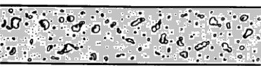
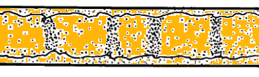
Excerpt from "CFD modeling of annular flow for prediction of the liquid film behaviour" by MARIA CAMACHO: "Annular flow is characterized by gas flowing as a continuous phase in the middle of a channel while liquid is present as dispersed droplets in the gas and as a liquid film at the walls of the surface. The liquid film mass is constantly changing due to three main interactions: deposition of liquid droplets onto the liquid film surface, liquid film evaporation on the liquid-gas interface and liquid film entrainment as droplets into the vapour flow." Mist flow: liquid phase is present only as dispersed droplets across the continuous vapour phase.
Discrete Phase Model: DPM
In Lagrangian particle tracking (Euler-Lagrangian approach), the discrete or dispersed phase comprises of particles and bubbles. While the term 'particle' is used to represent the dispersed phase, it inherently refers to a 'parcel' or 'agglomeration' or 'assemblage' of similar particles. Note: in ANSYS FLUENT, in steady-state discrete phase modeling, particles do not interact with each other and are tracked one at a time in the domain. Even when in reality droplets or solid particles are individual physical particles, ANSYS Fluent does not track each physical particle but groups of particles known as parcels. Thus, the model tracks a number of parcels, and each parcel is representative of a fraction of the total mass flow released in a time step. The number of "actual physical" particles in a parcel is adjusted in such a way that it satisfies the mass flow rate.Note that the results of DPM simulation is influenced by gravity when they have mass - for theoretically massless particles, gravity would not have any impact of the trajectories of the particles. Gravity leads to settling or sedimentation and is an important factor in modeling of cyclone separators and spray dryers. Default shape of particles are spherical and approximations are required for non-spherical particles (such as cylinders, capsules, pucks or disks, ellipsoids and thin sheets) as spherical particles with equivalent drag characteristics using appropriate drag laws.
For DPM, why both velocity and mass flow rate be defined in particle injection? As per article "innovationspace.ansys.com/ ... /relationship-between-velocity-and-flow-rate-in-dpm", the standard approach "mass flow rate = density * velocity * cross-section area" does not hold true for particles as they do not occupy the entire cross-section.
In steady-state discrete phase modeling, particles do not interact with each other and are tracked one at a time in the domain.
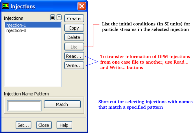
The primary inputs that a user must provide for DPM calculations are the initial conditions that define the starting positions, velocities, parameters for each particle stream and the physical effects acting on the particle streams. Initial conditions of a particle/droplet stream is specified by creating an 'injection' and by specifying its attributes. The initial conditions describe the instantaneous conditions of an individual particle which are:
- position (x, y, z coordinates) of the particles or parcels
- velocities (u, v, w) of the particle. For cone injections, velocity magnitudes and spray cone angle are used to define the initial velocities
- diameters of the particle
- temperature of the particle
- mass flow rate of the particle stream that will follow the trajectory of the individual particle/droplet though it is required only for coupled calculations
- additional parameters for special injections such as atomizer models
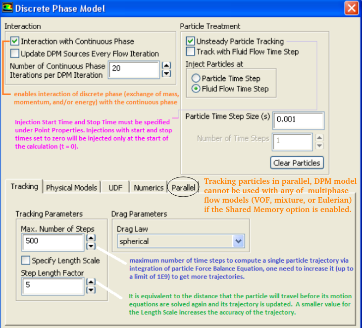
Max. Number of Steps: This factor is used to abort trajectory calculations when the particle never exits the flow domain. When the maximum number of steps is exceeded, Ansys Fluent abandons the trajectory calculation for the current particle injection and reports the trajectory fate as incomplete.
If the field "Number Of Continuous Phase Iterations Per DPM Iteration" field is set to 0, FLUENT will not perform any discrete phase iterations. Excerpts from ANSYS FLUENT: rule of thumb to follow when setting the parameters above is that if you want the particles to advance through a domain consisting of N mesh cells into the main flow direction, the Step Length Factor × N ≈ Max. Number of Steps.The particle positions are always computed when particles enter/leave a cell even if a very large length scale is specified. The time step used for integration will be such that the cell is traversed in one step.
Also, if "Number Of Continuous Phase Iterations Per DPM Iteration" field is reduced, the coupling between dispersed and continuous flow increases and vice-versa. For a closer coupling, this value should be set to a value ≤ 5 though no unique upper limit exists. Increasing the under-relaxation factor (setting value closer to 1) for discrete phase improves coupling and reducing the under-relaxation factor (setting value away from 1 and closer to 0) for discrete phase weakens the coupling.
DPM Trajectory Equation
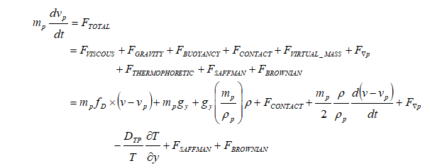
ANSYS FLUENT calculates drag coefficient of non-spherical particle using shape factor defined as [s/S] where 's' is the surface area of a hypothetical sphere having the same volume as the particle and 'S' is the actual surface area of the particle.
As explained above, the underlying physics of DPM is described by ordinary differential equations (ODE) as opposed to the Navier-Stokes equation for continuous flow which is expressed in the form of partial differential equations (PDE). Therefore, DPM can have its own numerical mechanisms and discretization schemes, which can be completely different from other numerics (such as discretization schemes) to solve the governing equations. The Numerics tab gives users control over the numerical schemes for particle tracking as well as solutions of heat and mass equations related to particles - continuous phase interactions.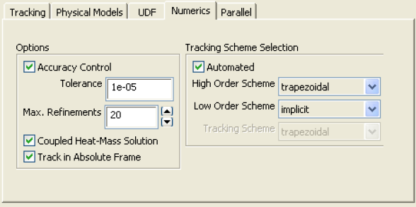
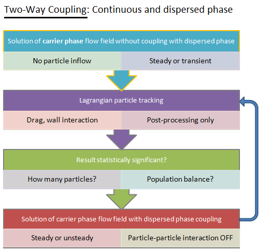
Type of coupling: continuous (carrier) phase and discrete phase
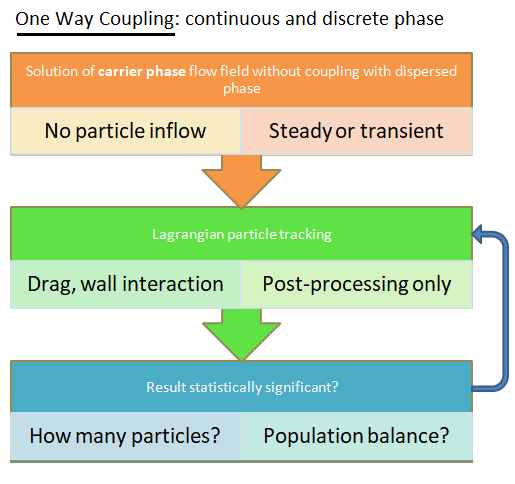
- no collisions at all (used for dilute suspensions): one-way or two-way coupling, Newton's equation of motion for dispersed phase.
- 3-way coupling - soft-sphere approach (the discrete element method, DEM): the instantaneous inter-particle contact forces due to oblique collisions (the normal, damping and sliding forces) are computed using equivalent mechanical elements springs, dashpots and sliders respectively. This approach requires a very small time step which can be as low as < 1 [μs].
- 3-way coupling - hard-sphere approach: interactions between particles are pair-wise (binary collision), instantaneous, momentum-conserving. Faster than soft-sphere method due to feasibility to use longer time steps.
In ANSYS FLUENT, the DDPM option is available only under Eulerian multi-phase model.
Type of Particle Injections
For typical applications, the computational cost of tracking all of the particles individually is prohibitive. Instead, the approach adopted in DPM and Discrete Element Method (DEM) Collision Model is that like particles are divided into parcels and then the position of each parcel is determined by tracking a single representative particle. Thus, in such calculations, following differences between DPM and DEM are mentioned in FLUENT user manual.- The mass used in the DEM calculations of the collisions is that of the entire parcel, not just that of the single representative particle.
- The radius of the DEM parcel is that of a sphere whose volume is the mass of the entire parcel divided by the particle density.
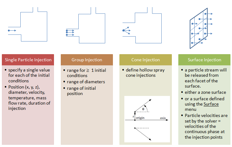
Group injections requires to set the properties position, velocity, diameter, temperature and and flow rate for the First Point (φ1) and Last Point (φN) in the group. ANSYS FLUENT assigns a value of φi to the i-th injection in the group using a linear variation between the first and last values for φ. The specified flow rate is defined per particle stream and can also be interpolated linearly between mass flow rates of the first and last injection points.
In ANSYS FLUENT, particle initial conditions (position, velocity, diameter, temperature and mass flow rate) can also be read from an external file to describe injection distribution. The file has the following form with all of the parameters in SI units. All variables inside the parentheses are required, name is optional.
(( x y z u v w diameter temperature mass-flow) name)
Sample files generated during sampling of trajectories (path Reports → Sample → Set-up...) for steady particles can also be used as injection files since they have a similar file format. Note that one line in the file = one parcel, 10 lines in the file = 10 parcels, 100 lines in the file = 100 parcels ... "parcels" = groups of particles which have similar properties (diameter, velocity, temperature) as each particle. Parcels are used as computationally it is impossible to track very large number say millions of particles. The mass-flow of the parcel = mass-flow of the group of particles. Generally the more parcels you use, the more accurate the solution shall be.
Mass flow rate: Only for coupled calculations (discrete phase affecting flow field of continuous phase), the mass of particles per unit time that follows the trajectory can be defined in the injection setting option. Also note that the number of streams (say 100) is not the same as the number of particles. The DPM uses a parcel method where many particles are tracked in each parcel and ANSYS FLUENT allocates the number of particles in each parcel based on the particle diameter, density and mass flow rate. Number of particles in each parcel NP = mPS × Δt / mP where mPS = mass flow rate in particle stream, mP = mass of each particle and Δt is the time step. Under steady state operations, it is assumed that any particle released from the same location with the same conditions will follow the same trajectory. P_FLOW_RATE macro can be used in a UDF to return the flow rate of a parcel in [kg/s].
Example: particle release from a surface - assuming there are 200 faces in the surface.
- The particle injected is sand with density of 2000 [kg/m3] and diameter 250 [μm]. Thus, mass of each particle is 8.18 [μg]
- Total mass flow rate of sand particles = 0.1 [kg/s].
- Total number of particles = 0.10 [kg/s] / 8.18×10⁻⁹ [kg] = 1.22×10⁹ [particles/s]
- Thus, the 200 trajectories releases from 200 faces of the surface represents 1.22×10⁹ actual [particles/s].
- If one defines a range of diameters by specifying "minimum diameter", "maximum diameter" and "number of diameters", the total number of trajectories computed will increase to 200 × "number of diameters".
- If stochastic tracking is switched on to account for Turbulent Dispersion and number of tries specified is 20, now the total number of trajectories computed will be 200 × "number of diameters" × "number of tries".
Number of Particle Streams: This option controls the number of droplet parcels that are introduced into the domain at every time step.
Note the options at top right quadrant of "Discrete Phase Model" setting window: Inject particles at (i)Particle Time Step and (ii)Fluid Flow Time Step. The option (i) requires two entries (a)Particle Time Step Size in [s] and (b) Number of Time Steps. Option (ii) requires only (a) Particle Time Step Size. To start the particle injection at t = 0, set "Start Time" of inject = 0. In order to keep the particle injection long after the time period of interest, set a large value for the Stop Time, for example 500 [s] which ensures that the injection will essentially never stop.Estimation of Number of Particles in Injections for DPM
Following calculator can be used to estimate the number of particles of specified diameter required to generate a known mass flow rate.| Diameter of the droplets: DP [μm] | |
| Density of the particles: ρ [kg/m3] | |
| Mass flow rate [kg/s] | |
| Velocity of particles [m/s] | |
| Number of trajectories [-] | |
Poincaré plots are made by placing a dot on a given surface every time a particle trajectory hits or crosses that surface.
In ANSYS FLUENT, particles can be tracked and their status to be written to files when they encounter selected surfaces. ANSYS FLUENT had options to write particle states (position, velocity, diameter, temperature, and mass flow rate) to files at various boundaries and planes (lines in 2D) using the Sample Trajectories Dialog Box. Sampling of DPM particles can be used to get the information of particles passing through the boundary and can be written to a text file. Report -> Discrete Phase -> Sample: Select the injection in "Release from Injection" tab, then select a face from Boundaries or Plane and then Click Compute. A file called 'surface.dpm' gets created in the working directory.
"File -> Export -> Particle History Data..." can be used to save injection tracking data. In CFD-Post: File -> Import -> Import FLUENT Particle Track File can be used read the data. For unsteady particle tracking, the particle trajectories will be updated and the particle states will be written to the files as they cross the selected planes or boundaries. Erosion and accretion rates can be accumulated for repeated trajectory calculations as described below.
Display the location of particles or volume fraction using DPM in ANSYS Fluent: 1) Turn on "Interactions with continuous phase" in the Discrete Phase Models window 2)Enable "data sampling for statistics" in "Run calculations" tab, then enable "DPM variables" in "Sampling options..." 3)Create the contour plot on a plane or boundary surface by selecting the option "Discrete Phase Variables" and the "DPM volume fraction" in the drop-down list.
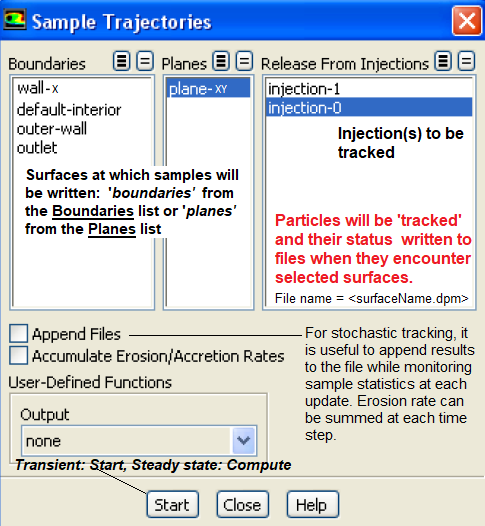
Total number of parcels, Total number of particles, Total mass, Maximum RMS distance from injector, Maximum particle diameter, Minimum particle diameter, Overall RR Spread Parameter, Maximum Error in RR fit, Overall RR diameter, Overall mean diameter (D10) - Comparisons / evaporation, Overall mean surface area (D20) - Absorption, Overall mean volume (D30) - Hydrology, Overall surface diameter (D21) - Adsorption, Overall volume diameter (D31) - Evaporation / molecular diffusion, Overall Sauter diameter (D32) - Combustion / mass transfer / efficiency studies and Overall De Brouckere diameter (D43) - Combustion equilibrium.
During steady DPM trajectory calculations in Fluent, if the maximum number of steps are reached and some particles still do not end up to the outlet (or escape/trap boundary), the status of such particles are reported as 'incomplete'. To avoid a large number of incomplete particles, it is suggested to increase the value of "Max. Number of Steps" in the DPM panel. If increasing the number of maximum steps still results in a large number of incomplete particles,
- Check if re-circulation regions are present in the solution domain. If yes, it is likely that particles kept churning in such region and are not able to reach exit of the domain, thus reported as incomplete.
- High number of incomplete particles may also be caused by flow field not fully converged. In such a case, it is recommended to make the flow converge without DPM, then inject the particles for DPM.
- Most of the time, high number of incomplete particles affect the convergence and speed of the DPM calculation. Therefore, a lower number of incomplete particles is desirable.
Injection from a File
Many a time, surface injection does not generate desired number of trajectories if the mesh is coarse. Injection from a file can be used where the injection points are generated by some other program. It is expected that a 'random' point generation method may yield a 'visually' uniform distribution of the points inside a disk. However, the probability function for distance 'r' from the center of a point picked at random in a unit disk is P(r)= 2.r and hence the point generated will be distributed as shown below.
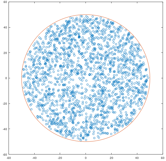
The GNU OCTAVE script used to generate it is as follows.
| % Data - number of points, radius, centre of the circle |
| n = 2000; RR = 50; xc = 0; yc = 0; |
| % Random angular cocordinates |
| q = rand(1, n) * (2*pi); r = rand(1, n) * RR * RR; |
| x = xc + 0.98 * sqrt(r) .* cos(q); |
| y = yc + 0.98 * sqrt(r) .* sin(q); |
| a = linspace(0, 2*pi, 100); |
| cx = RR * cos(a); cy = RR * sin(a); |
| figure(); hold on; box on; |
| plot(x, y, 'o'); % Plot the data points |
| plot(cx, cy, '-'); % Plot the boundary |
| hold off; |
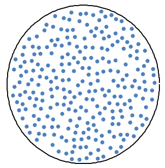
A Python program to generate the relatively uniform distribution of points based on spirals originating from the centre of the disk is summarized below. Reference: stackoverflow.com/ questions/ 27606079/ method-to-uniformly-randomly-populate-a-disk-with-points-in-python
| import math |
| import random |
| import numpy as np |
| import matplotlib.pyplot as plt |
| n = 2000 |
| R = 50 |
| alpha = math.pi * (3 - math.sqrt(5)) #The "golden angle" |
| phi = random.random() * 2 * math.pi |
| x = np.empty((n,1)) |
| y = np.empty((n,1)) |
| for k in range(1, n): |
| q = k * alpha + phi |
| r = math.sqrt(float(k)/n) |
| x[k-1] = 0.98 * R * r * math.cos(q) |
| y[k-1] = 0.98 * R * r * math.sin(q) |
| # for plotting circle line: |
| a = np.linspace(0, 2*np.pi, 100) |
| cx,cy = R * np.cos(a), R * np.sin(a) |
| fg, ax = plt.subplots(1, 1) |
| ax.plot(cx, cy,'-', alpha=0.5) #Draw circle boundary |
| ax.plot(x, y, '.') #Plot points |
| ax.axis('square') |
| plt.xlim(-R*1.05, R*1.05) |
| plt.ylim(-R*1.05, R*1.05) |
| plt.show() |
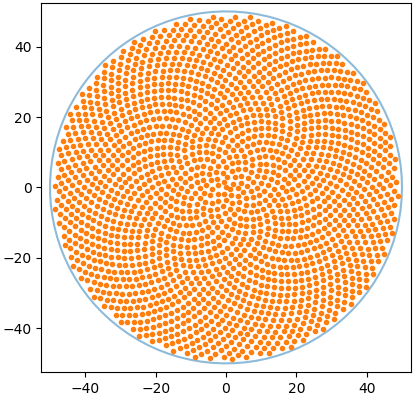
The recommended option is to independently mesh the injection plane and extract centroid of the triangles. This can be achieved by importing the vertices of the triangular elements and finding their centroid as arithmetic average of the coordinates. In ANSYS FLUENT, one may use the following UDF on demand to write centroids of the faces of a boundary zone in a text file.
#include"udf.h"
FILE *fout;
float fc[ND_ND]; /*Array to store X-, Y- and Z-Coordinates */
DEFINE_ON_DEMAND(getCentroidCoords) {
  Domain *domain;
  face_t f;
  Thread *t_face;
  domain = Get_Domain(1);

  /* Change boundary zone ID '2' as per your requirement */
  t_face = Lookup_Thread(domain, 2);
  fout=fopen("faceCentroids.txt", "w");

  if (fout == NULL) {
    Message("The text file cannot be opened for writing!");
  }
  else {
    begin_f_loop(f, t_face) {
      F_CENTROID(fc, f, t_face);
      fprintf(fout,"%g %g %g \n", fc[0], fc[1], fc[2]);
    }
    end_f_loop(f, t_face)
  fclose(fout);
  }
}
TUI Commands for Particle Injection in FLUENT
/define/injection/create-injection inj-inlet-x no (Particle Type [inert]: Change current value?) surface (type of injection) no (Injection material [Anthracite]: change current value?) z-inlet (surface name for injection) () yes (Scale Flow Rate by Face Area) yes (Use Face Normal for Velocity Components) yes (Stochastic Tracking?) no (Random eddy Lifetime?) 5 (Number of Tries) 0.15 (Time Scale Constant) no (Modify Laws?) no (Set user defined initialization function?) no (Cloud Tracking?) no (Rosin Rammlar diameter distribution) 0.1 (Diameter [mm]) 25 (Temperature [C]) 5 (Velocity magnitude [m/s]) 0.005 (Total Flow Rate [kg/s]) - note that all Units are as per those defined through Units -> Set Units tab. Thus, a typical TUI command would be: /define/injection/create-injection inj-inlet-x no surface no z-inlet () yes yes yes no 5 0.15 no no no no 0.1 25 5 0.005
define injections set-injection-properties can be used to edit an existing particle injection definition. To track: /solve/dpm-update. To print summary: /report/dpm-summary. /solve/initialize dpm-reset: Reset discrete phase source terms to zero.f To plot the particle track of an injection: [Create] display objects create particle-tracks p-track-x field particle-resid-time () [Select injection] display objects edit p-track-x injections-list inj-inlet-x () q [Define colourmap] display object edit p-track-x color-map color rgb [Define color band] display object edit p-track-x color-map size 10 [Display Track] display object display p-track-x
Create Injection by a Point: surface/point-surface point_1 0.2 0.5 0.2, define/injections/create injection-001 n y surface n point_1 n n n n n n 0 0 0 1e-06 0. These two commands can be put in a loop to read point coordinates from a text file and create injection for each of those points.
Report DPM summary to a file:
/display/set particle-tracks display? no
/display/set particle-tracks report-type summary
/display/set particle-tracks report-to file
/display/set/particle-tracks report-type step
/display/set/particle-tracks history-filename "dpm.txt"
/display/set/particle-tracks/report-variables particle-mass
 particle-x-position particle-y-position particle-z-position
 particle-reynolds-number particle-temperature q
/display/objects/particle-tracks particle-track-1 particle-resid-time
 injection_0 () 0 5
Particle Sampling: /report/dpm-sample/injection_0 () () plane-xy () no no: this is to start taking the sample. solve/iterate 1000, /report/dpm-sample: this is to stop sampling. In case an UDF is used, a generic form of TUI command would be: /report/dpm-sample injection-name () boundary-location () sample-plane () UDF-name no. In case sampling is to be done either on a boundary location or a sample plane, they can be ignore but () must be retained. Following is an example to copy injection settings:
define/injections/set-inj-prop injection-0 injection-1
Particle type [inert]: Change current value? [no] no
Injection type [surface]: Change current value? [no] no
Injection Material [dpm]: Change current value? [no] no
Number of Streams [10000] 5000
Available surfaces: (fluid-x fluid-z b_inlet int-x)
Chosen: (b_inlet)
Surface(1) [b_inlet]
Surface(2) [()]
Use Face Normal for Velocity Components: [yes] yes
Stochastic Tracking? [yes] yes
Random Eddy Lifetime? [no] no
Number of Tries [2] 3
Time Scale Constant [0.015] 0.025
Modify Laws? [no] no
Set user defined initialization function? [no] no
Cloud Tracking? [no] no
Rosin Rammler diameter distribution? [no] no
Diameter in ([mm]) [0.5] 0.1
Temperature in ([C]) [25] 50
Velocity magnitude (in [m/s]) [2.5] 5.0
Total flow rate (in [kg/s]) [0.75] 0.10
Parcel Depletion Model in STAR-CCM+:This model allows removal of parcels from the simulation based on specified criterion when they are no longer relevant or important. For example, parcels can be removed based on their residence time, distance travelled, mass fraction, or other properties. By doing so, the number of parcels and the size of the track file can be reduced without compromising the accuracy of the simulation.
Dense Discrete Phase Model
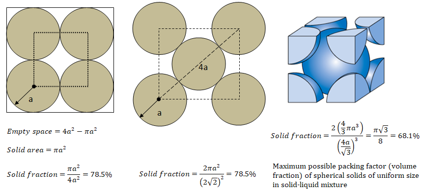
ps = [1+2(1 + e) α gr ]α ρp Θs
where e is the coefficient of restitution, gr is the radial distribution function - a correction factor that modifies the probability of collisions between grains when the solid granular phase becomes dense (may also be interpreted as the non-dimensional distance between spheres), α is the volume fraction of solid, ρp is the density of solid particles and Θs is the granular temperature. The radial function tends to infinity as the volume fraction tends to the packing limit and it tends to 1 as the volume fraction approached zero (the dilute limit).The term "granular temperature" has been borrowed from kinetic theory of gases and is a bit misnomer which does not represent any temperature in thermodynamic sense. It represents particle momentum exchange due to translation and collision leading to definition of kinetic and collisional viscosities respectively. The shear and bulk viscosities arising due to this phenomena is added to the solid stress tensor. The granular temperature for the solids phase is proportional to the kinetic energy of the particles’ random motion mathematically expression as Θs = 1/3[u'.u'] where u' is the fluctuating solids velocity in the Cartesian coordinate system. This is defined as an ensemble average of the particles’ random velocity within a finite volume and time period having particle number per unit volume as averaging basis.
The collisional part of shear viscosity: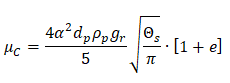
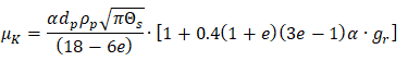
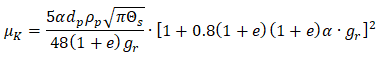
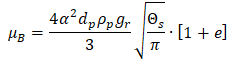
Eulerian Wall Film
A wall film is a thin layer of liquid over a solid surface such as water dripping due to condensation. The surface tension is one of the dominant parameter which controls the thickness and flow rate of such liquid films. The Eulerian Wall Film (EWF) model can be used to predict the creation and flow of thin liquid films on the surface of walls. The thin film assumption is one usually made in both Eulerian and Lagrangian film modeling approaches, specifically that the thickness of the- film is small compared to the radius of curvature of the surface so that the properties do not vary across the thickness of the film and
- films formed are thin enough so that the liquid flow in the film can be considered parallel to the wall, with an assumed quadratic shape.

- stick: where the droplet impacts the wall with little energy and remains nearly spherical
- rebound: where the drop leaves the surface relatively intact but with changed velocity
- spread: where the drop hits the wall with moderate energy and spreads out into the film and
- splash: where part of the impinging drop joins the film and another part of the drop leaves the wall in several other smaller drops.
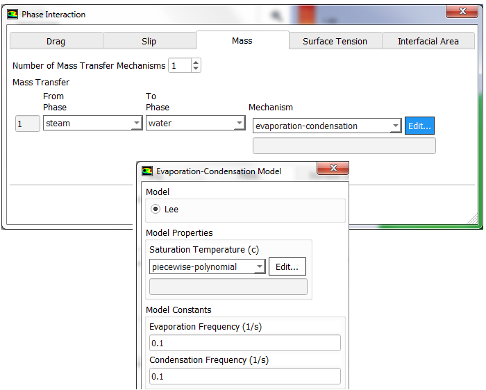
Advanced Solver Setting: AMG
The Algebraic Multi Grid solver is one among the family of multi-grid solvers. The adjective multi-grid refers to the concept that the solution process is implemented more than one grid (levels) even though the user has created only one grid.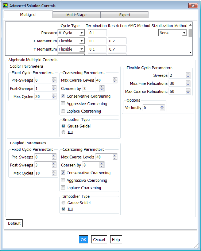
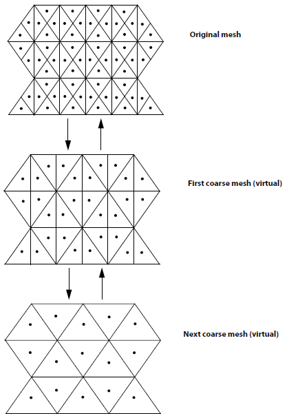
Transient Table as Boundary Condition in FLUENT
A time-history data such as inlet temperature as function of time or mass flow rate as function of time can be specified either as an UDF (cases where analytical equations can be derived) or as a data table.The format of the standard transient profile file:
(
 (inletvel transdata 3 0)
 (time  1 2 3 )
 (invel 6 5 4 )
)
Here '3' denotes the number of data points (number of rows in tabular format). '0' indicated that data is not time-periodic, use '1' for a time-periodic dataset. 'invel' shall appear as drop-down in boundary condition panel. Note:
- All quantities, including coordinate values, must be specified in SI units.
- Profile names (e.g. 'inletvel' in this example) must have all lowercase letters
- Data can be either in column or row format.
The data set used above can also be specified as described below:
(
 (inletvel transdata 3 0)
 (time
  1
  2
  3
 )
 (invel
  6
  5
  4
 )
)
Tabular Transient Profiles
The format of the tabular transient profile file is as follows. Use TUI command "file read-transient-table fileTr.dat" to upload the data into the solver. The options "inletvel time", "inletvel invel" and "inletvel outpr" shall appear in the drop-down menu of boundary condition panels. The entry '4' indicates number of fields, '3' indicates number of data rows, '0' means data is not "time-periodic". Change 0 to 1 for time-periodic data which means the values shall get repeated after number of rows specified. All quantities, including coordinate values, must be specified in SI units because ANSYS FLUENT does not perform unit conversion when reading profile files. Also, profile names must have all lowercase letters.inletvel 4 3 0 time invel outpr hs 1 6 0 50 2 5 1000 250 3 4 2000 500The first field name should be used for the 'time' field, which represents the flow time, must be in ascending order. When entering the number of variables, avoid having any extra spaces before or after the numbers especially when the local machine and remote machine are using different operating systems. The newline characters for text files are different on the two OS: in Linux it is \n and in Windows it is \r\n. Notepad++ supports automatic conversion of EOL format to Unix: Edit > EOL Conversion > Unix (LF). On Windows machine, run Linux binaries from the Windows Command Prompt (CMD) or PowerShell using wsl. For example: C:\Users> wsl ls -la. Similarly, wsl dos2unix win_format.txt can be used to convert the text file compatible to Linux OS.
Data Sampling in Transient Runs
To calculate mean values and Root Mean Square Error (RMSE) of field variables over specified number of time steps in transient run, use the following settings.

Interpolation of Results
Many a times we need to interpolate the results from previous simulations into a new simulation, such as when a new mesh is generated due to refinement or coarsening. Sometimes results may be available from simulations carried out in other software (such as FLUENT or OpenFOAM) and the field variables need to be read into a new software (STAR-CCM+). Most of the commercial program provide an options to import and export data from and into CGNS and/or CSV format. The data in this format can be used to exchange result data from one program to the other.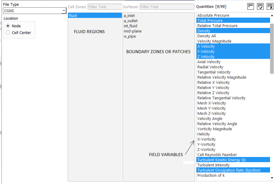
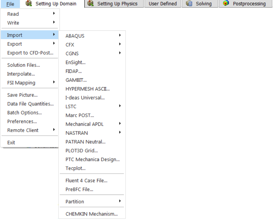
Interpolation file format: ANSYS FLUENT
2            --the interpolation file version
3            --dimension (2 or 3)
25000        --total number of points
3            --total number of fields (velocity, pressure...) included
x-velocity   --field variable to be interpolated
pressure     --field variable to be interpolated
-0.100000    --x-coordinate of first node in the list
-0.200000    --y-coordinate of first node in the list
-0.300000    --z-coordinate of first node in the list
  ...
  ...
  ...
 1.000000    --x-coordinate of last node in the list
 2.000000    --y-coordinate of last node in the list
 3.000000    --z-coordinate of last node in the list
 0.500000    --x-velocity at first node in the list
 0.100000    --x-velocity at second node in the list
 0.200000    --x-velocity at third node in the list
  ...
  ...
  ...
 5.000000    --x-velocity at last node in the list
 100.0000    --pressure at first node in the list
 200.0000    --pressure at second node in the list
 300.0000    --pressure at third node in the list
  ...
  ...
 500.0000    --pressure at last node in the list
At the end is a list of the field values at all the points in the same order as their names. The number of coordinate and field points (x-velocity and pressure in this case) should match the number given in line 3 (25000 in this case). Note that it cannot interpolate heat generation rate (W/m3), though internal energy, enthalpy, heat transfer coefficient... can be interpolated. In other words, no volumetric source/sink term can be interpolated in the fluid region. On the boundaries, all field variables are available for interpolation.
Data Export into CSV Format: ANSYS FLUENT:
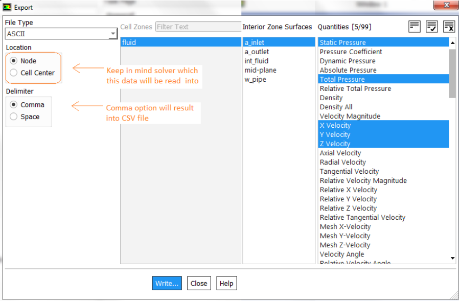
The header in CSV files for FLUENT and STAR-CCM+ uses different variable names. In STAR-CCM+ variables has to be specified with appropriate units: e.g. "Absolute Pressure (Pa)", "Velocity Magnitude (m/s)", "Velocity[i] (m/s)", "Velocity[j] (m/s)", "Velocity[k] (m/s)", "X (m)", "Y (m)", "Z (m)"... Note the space between variables and unit. The x-component of velocity is accessed by Velocity[i].
Data Mapper: STAR-CCM+:
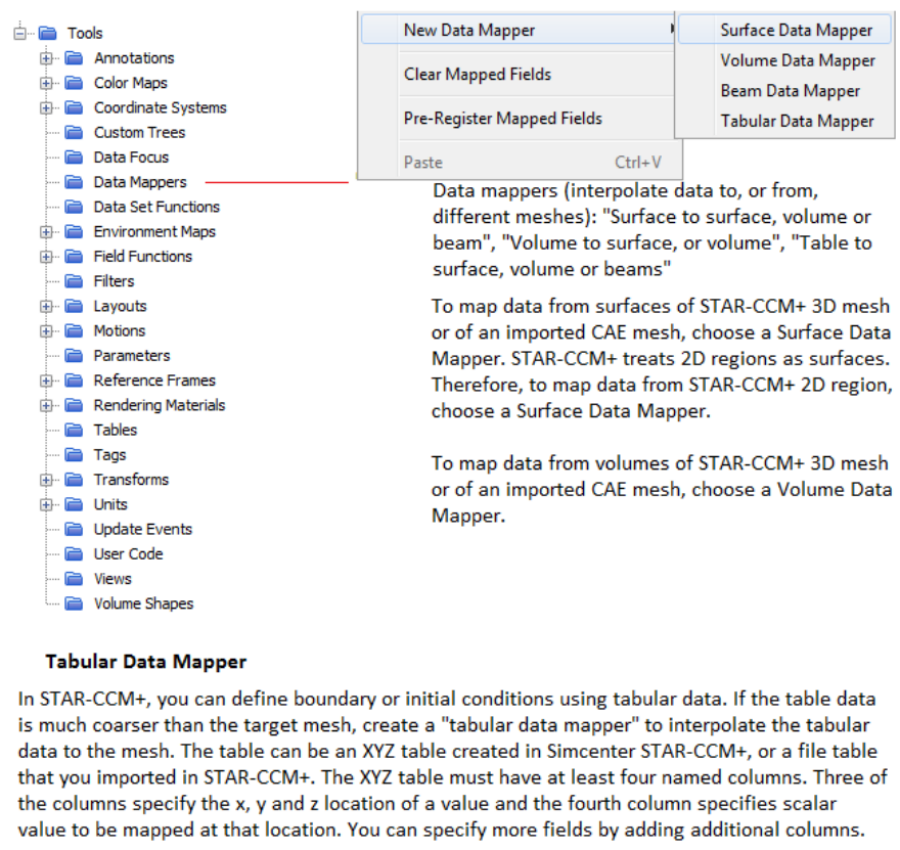
interpolateTable(@Table("VelData"), "Time", LINEAR, "VelMPS", $Time)
Here the field function type should be vector. For boundaries such as inlet, in the “Physics Values” option of the boundary in the “Method” field, select Field Function, and then right below this, select the field function defined earlier.
The name of the table is VelData, Time is the name for the first column in the .csv file, LINEAR (other option available is SPLINE) is the interpolation method creating values between the discrete time values specified in the table, VelMPS is the name of the second column in the table (corresponding to the velocity magnitude), $Time specifies that the velocity is function of time. In case velocity is function of spatial coordinates say y-axis: $${Position}[1] can be used in place of $Time to specify that the position coordinate is aligned with the y-axis (1 = y-direction, use '0' for x-direction and 2 for z-direction).
Auto-save Intermediate Results
Solver can automatically save case and data files at specified intervals during a calculation. This is recommended for all type of solutions and is especially useful (necessary) for time-dependent calculations, where is is required to save the results at different time steps or flow times without stopping the calculation and performing the save manually. Intermediate result files can be used also for debugging or troubleshooting poor convergence, incorrect result... In ANSYS FLUENT, if the specified 'root' file name ends in .gz or .Z or h5, appropriate file compression is performed during auto-save. The compression can be performed manually also once the data is saved in uncompressed format. From website of TotalComress: "TotalCompress is a multi-core compression tool which can compress results 120 times faster than legacy compression tools by utilizing multiple CPU cores with an optimized parallel algorithm." In STAR-CCM+ the zip/unzip operations have to be performed using command line while making runs on a cluster.Automatic Numbering of Files
- For transient calculations, to save files with names that reflect the time step at which they are saved: include the character string %t in the file name. For example, with case_%t.dat.h5 for the file name, solver saves a file with the name case_0050.dat.h5 if the solution is at the 50 time step. This automatic saving of files with the time step should not be used for steady-state cases, since the time step will always remain zero.
- For transient calculations, to save files with names that reflect the flow-time at which they are saved, include the character string %f in the file name similar to %t. By default, the flow-time thus included in the file name will have a field width of 10 and 6 decimal places. To modify this format, use the character string %x.y f, where x and y are the preferred field width and number of decimal places, respectively. ANSYS FLUENT will automatically add zeros to the beginning of the flow-time to achieve the prescribed field width. To eliminate these zeros and left align the flow-time, use the character string %-x.y f instead.
- To save a file with a name that reflects the iteration at which it is saved, use the character string %I in the file name. For example, case_%i.dat.h5 saves a file with name case_0500.dat.h5 after 500 iterations.
- To save a picture file with a name that reflects the total number of picture files saved so far in the current solver session, use the character string %n in the file name. This option can be used only for picture files.
- The default field width for %I, %t, and %n formats is 4 which can be changed by using % xi, %xt, and %xn in the file name, where x is the preferred field width such %10i or %5t.
Parametric Study in FLUENT
A parametric study such can include not only geometrical changes but just changes in boundary conditions, material properties and solver type for a fixed geometry and mesh. Following screenshots describes steps to make such study. To create parameters through the TUI, the following option needs to be enabled: /define/parameters/enable-in-TUI? yes. The parametric study in stand-alone FLUENT session can handle only boundary conditions and not geometrical changes. To study impact of geometrical changes, ANSYS Workbench would be required where parameters can be defined in Ansys Discovery. The user of Ruler option under Pull operation in Discovery is a common method to specify geometrical parameters.

To know how to create a Design of Expriment (DOE) table, refer to this section.

- First Step: Create a case that gives reasonable correct results setting the boundary conditions as 'fixed-type'.
- Next Step: Change the desired boundary to parameters by selecting "New input Parameter" by opening the drop-down through the downwards arrow in the Boundary Condition Condition panel.
- Next Step: Under the 'Parametric' tab, click Add Design Point 1-2 times and export it to a csv file.
- Edit the values in the csv file and add extra rows as needed.
- Once all the combinations of parameters (DOE table) is set, re-import this into Fluent.
- Create a report item in the Report Definitions under Solution and tick "Create Output Parameter" so that they appear on the Parametric Study tab.
- As the baseline case ran successfully, the Update All button should run successfully though not guaranteed to converge.

TUI commands for Parametric Studies in ANSYS FLUENT
The link parametric.fluent.docs.pyansys.com/dev/examples/00-parametric/index.html provides a Python-based example. It can be converted to a journal-based by converting Python statements into Scheme/TUI commands./parametric-study/study initialize yes , /parametric-study/design-points add no yesHere 'no yes' on the last statement is response to queries "Do you want to write data?" and "Do you want to capture simulation report data?".
Enable parameter creation in the TUI: "define parameters enable-in-TUI yes". Create input parameters: "define/b-c/set/velocity_inlet inlet-x () vmag yes par_in_vel 1.5 q" and "define/boundary-conditions/set/velocity-inlet inlet-x () temperature yes par_in_temp 300 q".

Format of a .csv Design Point Input Table
| Name | par_in_vel | par_in_temp | Write Data | Capture Simulation Report Data | Status |
| Units | [m/s] | [C] | |||
| DP_0 | 5 | 75 | Yes | No | Need Update |
| DP_1 | 2 | 50 | Yes | No | Need Update |
| DP_2 | 1 | 25 | Yes | No | Need Update |
The csv file shall have the format shown below. More columns can be added to introduce new input parameters and new rows can be added to increase number of design points.
Name, par_in_vel, par_in_temp, Write Data, Capture Simulation Report Data, Status
Units, [m/s], [C]
DP_0, 5, 75, Yes, No, Need Update
DP_1, 2, 50, Yes, No, Need Update
DP_2, 1, 25, Yes, No, Need Update
Note that the runs may diverge if a solution of new design point is started with results from previous design point. For parametric study, it is advised to initialize the solution for every design point.
Parametric Study in CFX
Refer "Chapter 13: Operating Maps and Operating Point Cases" of "Ansys CFX-Solver Modeling Guide" and "Establishing Table Data and Creating Table Functions" in the "CFX-Pre User's Guide."An operating point case definition can be held by either: (a) An .mdef file and its supporting files, such as a table file (defining operating points) or (b) An .mres file and its supporting files, such as: – a table file (defining operating points) – results files for partially / fully completed operating point jobs (each job simulates a single operating point).
SPH: Smoothed-Particle Hydrodynamics
Available in STAR-CCM+ and ParticleWorks, commonly used in powertrain and drivetrain (gearbox) lubrications - does not require volume mesh and handles easily complex body motion and geometries. Tutorial on Gearbox lubrication using SPH added in V2402, additional license required in STAR-CCM+ to run the SPH solver.FSI: Fluid-Structure Interaction in ANSYS
FSI has wide application to check the effect of fluid forces on structural components such tank sloshing, flapping of wings and helicopter blades, pouring of liquid from a non-rigid container, pressure-limiting valves, leakage in fuel injectors operating at high pressure (such as Diesel engines) and check valves (deformable flow control devices) to name few.FSI simulations are classified under a broader category of "Multi-physics Simulations" and not limited only to structural simulations. Fluid-thermal interaction, Fluid-thermal-electric interaction, Fluid-piezoelectric interaction, Structural-magnetic interaction ... are other types of multi-physics simulations.
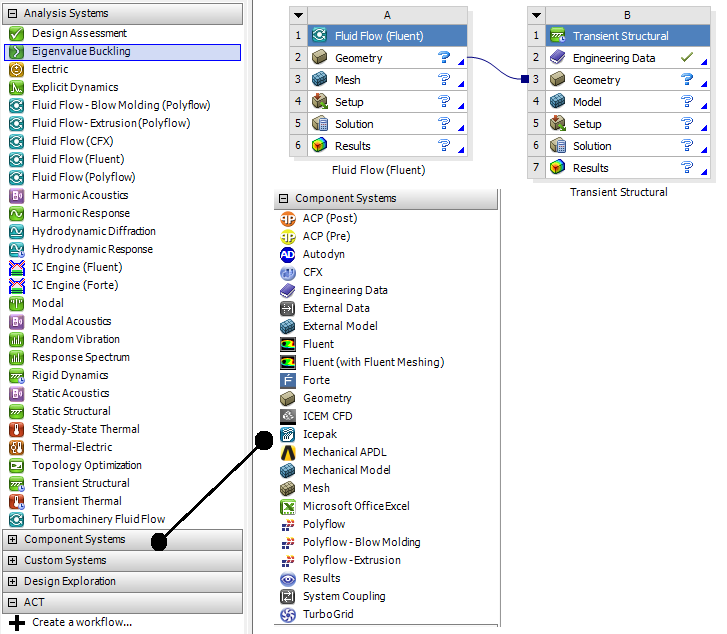
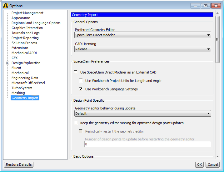
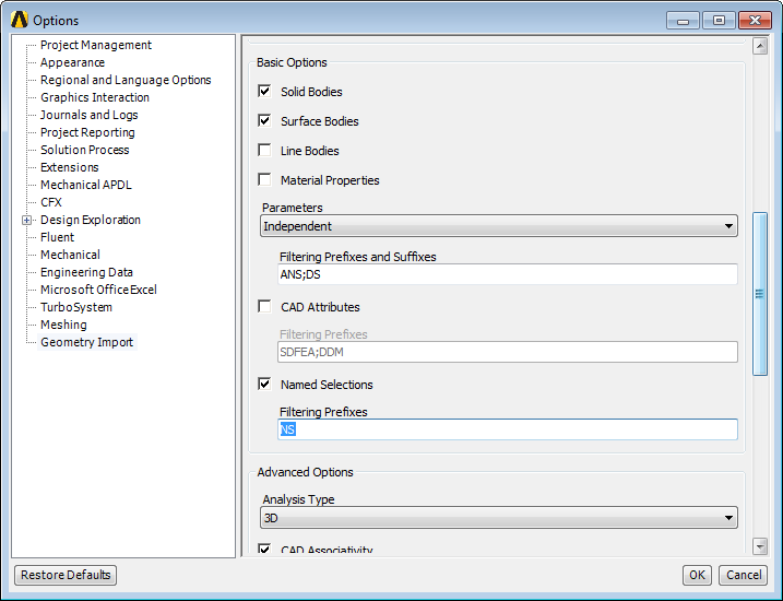
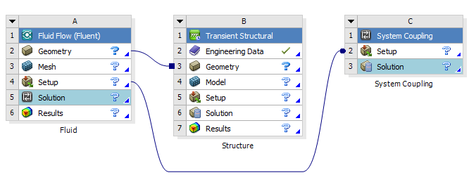
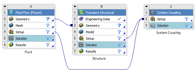
- Solution update can be done through System Coupling component only.
- System Coupling component overrides few settings in participant solver so that the time duration and time step settings are consistent across all participant solvers.
- The surface of solid boundary in contact with fluids need to be set as "Fluid-Solid Interface"in Transient/Static Structural Model.
- In fluid solver such as FLUENT, the "System Coupling" option needs to be activated under "Dynamic Mesh" tab.
- For FLUENT, all regions of type 'Wall' are shown in System Coupling setup.
- For (Transient/Static) Mechanical, all regions of type "Fluid-Solid Interface" appear in System Coupling component.
- Create solid-fluid coupling: select a fluid (FLUENT) and solid (Mechanical) region pair (use Ctrl key for multiple selection) and select "Create Data Transfer" from right click pop-up menu.
- "Data Transfer" defines the Source (participant solver, deforming region and variable being transferred e.g. force, displacement), Target (participant solver, deforming region and variable being transferred e.g. force, incremental displacement) and Data Transfer Controls (data transfer frequency, under-relaxation factor and convergence).
- Post-processing a FSI result:
- Use 'Result' cell in Transient/Static Structural or Fluid Flow (FLUENT) for solver-specific post-processing
- Connect structural 'Solution' cell directly to FLUENT system 'Results' cell or (c)Add a 'Results' System (ANSYS CFD-Post) for unified post-processing of structural and fluid results.
Parallel Processing
In order to reduce the simulation run time, parallel processing methods have been developed where the arithmetic involved with matrices are broken into segments and assigned to different processors. Some of the the terms associated with this technology are described below. The image from "Optimising the Parallelisation of OpenFOAM Simulations" by Shannon Keough outlines the layout of various components in a cluster.
One consideration while selecting a parallel processing cluster is either to have a pay-as-you-use system (such as cloud service) or have an on-premises cluster which can be used as much as the queuing system allows. While the first one may seem cost effective requiring negligible investment, it is beneficial only for a team and simulations processes matured in nature (strict adherence of checklists and multiple peer reviews). It does not allows for mistakes, divergences, and frequent scope creep. Also, spliting the project cost into 'pre-post' and 'solution' cost has inherent uncertainties.
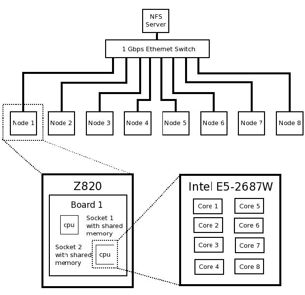
- HPC: High Performance Computing - A generic term used to describe the infrastructure (both hardware and software) for parallel processing.
- Cluster: A collection of workstations or nodes connected with each other with high speed network such as 1 GB/s Ethernet network or InfiniBand.
- Node: Each independent component of a cluster or HPC set-up. Each node has following configurations:
- Chassis: For example - HP Z820
- CPU: For example - Intel XEON-E5 2687W
- GPU: Graphics Processing Unit e.g. NVIDIA
- Cores: For example - 8 cores per CPU @ 3.1GHz
- RAM: For example - 8GB DDR3-1600 Registered ECC memory
- Storage: For example - 1TB SATA HDD plus network file system (NFS) server
- Operating System: For example - CentOS 6.5
- Application Program: For example - CFD Software: OpenFOAM or FLUENT V17.2
- Latency: it refers to dormant capacity or sluggishness of the cluster interconnect. In other workds, it also refers to the inertia of the system. Lesser the latency, faster the response time.
- Hyperthreading:It is a method which allows each core on the CPU to present itself to the operating system as two cores: one real and one virtual. The operating system can then assign jobs to the virtual cores and these jobs are run when the real core would otherwise be idle (such as during memory read/write) theoretically maximising the utilisation of the CPU. Excerpts from forum.ansys.com/forums/topic/problem-of-running-fluent-on-multiple-cpus: "Hyperthreading splits each node into two. ANSYS solvers are designed to fully utilise a node, so will use 100%. If the node is split each half will want to run at 100% so will fight, eventually it should settle at 50% each. However, you're now paying cpu costs for additional data traffic between nodes and for additional virtual cells on the parallel partitions. For Fluent if I double the number of nodes available I expect to half my iteration time. With hyperthreading I may see a 5-10% speed up depending on load balancing, I may see a 5% slow down. Given you are paying for the parallel licence it's not good value for money. The virtual CPU (turned on by hyperthreading) is treated the same as one physical CPU in terms of occupying the process limit by ANSYS license. ANSYS licence the solver process not the hardware: it is possible to run all 32 HPC licenses on a single physical core."
- Excerpts from STAR-CCM+ User Manual: "Generally, for best performance, it is recommended that you turn off any features that artificially increase the number of cores on a processor, such as hyperthreading. In situations where hyperthreading is turned on to benefit other applications, you should generally avoid loading more processes than there are physical cores.
In addition to turning off hyperthreading, it is recommended that you set your BIOS settings to favor performance rather than power saving. Almost all heavily parallelized applications suffer performance problems if the CPU frequencies are spun up and down. In most parallel applications and STAR-CCM+ in particular, when one core is operating at a reduced frequency, all other cores are running at lower frequencies as well.
- Excerpts from STAR-CCM+ User Manual: "Generally, for best performance, it is recommended that you turn off any features that artificially increase the number of cores on a processor, such as hyperthreading. In situations where hyperthreading is turned on to benefit other applications, you should generally avoid loading more processes than there are physical cores.
- Memory Intensive Applications: This refers to the programs whose performance is more influenced by RAM than the clock-speed of the CPU. For example - OpenFOAM
- Partitioning: This is nothing but a "work distribution" among CPUs. However, tracking of nodes and elements are important. Excerpts from FLUENT user's manual: "Balancing the partitions (equalizing the number of cells) ensures that each processor has an equal load and that the partitions will be ready to communicate at about the same time. Since communication between partitions can be a relatively time-consuming process, minimizing the number of interfaces can reduce the time associated with this data interchange."
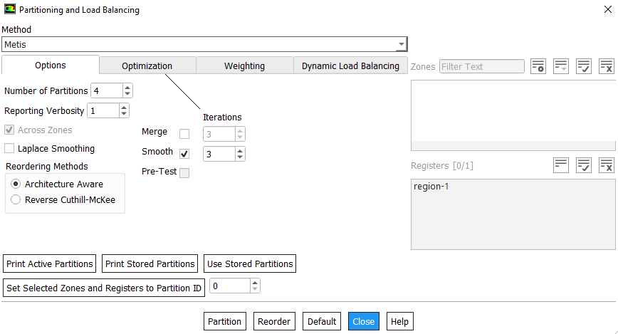
- MPI: Message Passing Interface - Each compute node is connected to every other compute node though the network and relies on inter-process communication to perform functions such as sending and receiving arrays, summations over all cells, assembling global matrix - remember A.x = b. Inter-process communication is managed by a message-passing library by an appropriate implementation of the Message Passing Interface (MPI) standard such as OpenMPI, Intel MPI, Cary MPI, IBM Platform MPI, Microsoft MPI, MPICH2 or vendor's own version of MPU.
- Scalability: It refers to decrease in turnaround time for solutions as the number of compute nodes increases. However, beyond a certain point the ratio of network communication time (refer to definition of Cluster above) to computational time increases, leading to reduced parallel efficiency, so optimal system sizing is important for any simulations - determined from a ratio of the time to compute and the time that is taken to exchange data between cluster nodes. Article docs.aws.amazon.com/ ... /cfd-case-scalability.html documents scalability in terms of number of cells per core.

- Bandwidth of overall cluster interconnect: In ANSYS FLUENT, a table containing information about the amount of data communicated within one second between two nodes can be printed to the console. The table summarizes the minimum and maximum bandwidth between two nodes. Checking the bandwidth is particularly useful when you cannot see good scalability with relatively large cases.
In ANSYS FLUENT, one can reduce communication and improve parallel performance by increasing the report interval for residual printing/plotting or other solution monitoring reports. The most relevant quantity is the Total wall clock time which can be used to gauge the parallel performance (speed up and efficiency) by comparing this quantity to that from the serial analysis. Alternatively, an approximation of parallel speed-up may be found in the ratio of Total CPU time to Total wall clock time.
The comparison of two machines or clusters should be made on following parameters:
| Design Parameter | Unit | Value-1 | Value-2 | Remark |
| CPU Operating Frequency | [GHz] | 3.5 | 4.2 | Base clock speed, base clock frequency |
| Maximum Turbo Frequency | [GHz] | 4.5 | 4.8 | Maximum Boost Clock |
| Instructions per clock | [M/cycle] | 3.5 | 3.2 | Parameter which decides actual computational speed |
| RAM size per core | [GB] | 4.0 | 6.0 | |
| Cache Memory Size | [MB] | 32 | 16 | Reduce time to access data from main memory |
| Bus speed | [GT/s] | 8.0 | 6.0 | |
| Interconnect Speed | [GB/s] | 100 | 80 | Such as infiniband |
| Hyperthreading? | [ - ] | Yes | No | No quantitative impact on computation speed |
Specification of a Workstation
| Speed: | 3.5 GHZ minimum |
| Storage: | 8 TB |
| HDD: | 3.5" 7200 RPM SATA |
| Memory: | 128 GB SO-DIMM DDR4 2400MHz |
| Display Type: | 24" LCD |
| Optical Drive: | Yes |
| Speaker: | with microphone |
| Graphics: | Integrated AMD Radeon Graphics or Quadro 580 |
| Camera: | Integrated |
| Networking: | Integrated 100/1000M |
| Keyboard: | Yes |
| Pointing Device: | USB Calliope Mouse, Black |
| WiFi Wireless LAN Adapters: | 11AC (2x2), Bluetooth 5.0 |
| Rear Ports: | 4xUSB 2.0, 1 x line-out (3.5mm), Ethernet (RJ-45), HDMI 1.4 |
| Front Ports: | 2xUSB 2.0, 2xUSB 3.2 Gen 1 |
| Headphone / microphone: | combo jack (3.5mm), 1xmicrophone (3.5mm) |
| Software Preload: | Windows 11 |
| MS-Office | 2020 |
Installation of Ansys Products
Excerpt from Ansys Installation Guide:All products available in the installation package(s) you downloaded are listed in a tree view. A checkmark to the left of the product signifies that the product and all related "child" products are enabled for installation while a grey box indicates that some, but not all products are enabled for installation. You can expand the tree to select any additional products you wish to install.
"The installation program attempts to query your license server to pre-select your installation options. If the query is successful, the following message is displayed: Review and change the pre-selected installation options if necessary. If the installation program was unable to query your license server, this message is not displayed and the default installation options are selected. You can select or deselect any combination of products. Ansys Workbench is automatically installed with most Ansys, Inc. products; there is no individual product selection for Ansys Workbench." Excerpt on Uninstallation: "Select the product(s) to be uninstalled and unconfigured and click Uninstall Selected Item(s). Not all products and product components may be listed individually."Making FLUENT Runs on Clusters
FLUENT runs on a cluster can be started either in [A] interactive mode (as if it is running on your local machine with all functionality of a GUI) or [B] in a batch mode with GUI OFF and graphics ON or [C] batch mode with GUI OFF and graphics OFF. In case of mode 'C', the runs can only be controlled and monitored either through text files and/or through FLUENT Remote Visualization interface. Note that the HPC server needs a trigger from the solver to stop or exit the job when there is any error while iterating. As per FLUENT user guide: "Batch option settings are not saved with case files. They are meant to apply for the duration of the current ANSYS FLUENT session only. As batch options are not saved with case files, journal files developed for use in batch mode should begin by enabling the desired batch option settings". The TUI command that should be added to the journal file before iterate statement is /file/set-batch-options n y y n where n, y, y and n stands for answer to "Confirm Overwrite?", "Exit on Error", "Hide Questions" and "Redisplay the Questions" respectively.From version 25R1 onwards, Fluent Remote Visualization is changed to Web Server: "/server/start-web-server remote_monitor , , ," is the TUI command to start the web server on the cluster. If not set-up correctly, it will throw error: "webserver/start-server: Webserver password not set in FLUENT_WEBSERVER_TOKEN environment variable."
Graphics refers to the pictures, videos, charts and animations. The graphics components of a computer control and enhance how these 'graphics' are displayed on computer screen. Usually the graphics components are on a separate card that is plugged into a slot on the motherboard though these can and are built directly into the motherboard as well. Some other names used for the graphics components are video card, video adapter and display adapter. NVIDIA Tesla GPUs for servers and workstations, Quadro GPUs for workstations and GeForce GPUs - gaming class cards are few examples of GPU.
Checkpointing - Save Intermediate Results: For some models, it may be needed to request multiple jobs in order to finish the convergence process and the [fixed interval] auto-save settings will not save state immediately prior to the job being terminated either manually or by the scheduler thus losing information. To address this there is an complimentary method which will save before your job finishes. Place the following commands in the journal file:
(set! checkpoint/check-filename "./check-fluent")(set! checkpoint/exit-filename "./exit-fluent").
This instructs solver to check for files called check-fluent and exit-fluent in the current working directory of the running job. The presence of check-fluent file will instruct Fluent to conduct a save and then resume computation. The presence of exit-fluent file will instruct Fluent to conduct a save and then exit. The exit-fluent command also automatically generates a #restart.inp file (a journal) which can be used to restart the job from where it was stopped.
GPU: Similar to an operating system which deals with how a computer starts and shuts down, the graphics driver is a program that enables computer to use the graphics card and communicate with CPU, HDD and other components. A 'driver' in general is a software component that lets the operating system and a 'device' communicate with each other. E.g. there is USB 'driver' to make a USB mouse work. The graphics card sends the signal to the computer display and makes the data visible.
Note that computer 'monitors' are not same as "graphics cards or graphics drivers". Graphics card is a hardware and graphics driver is software to make it work. AMD Radeon a graphics card used in my laptop manufactured by Lenovo. 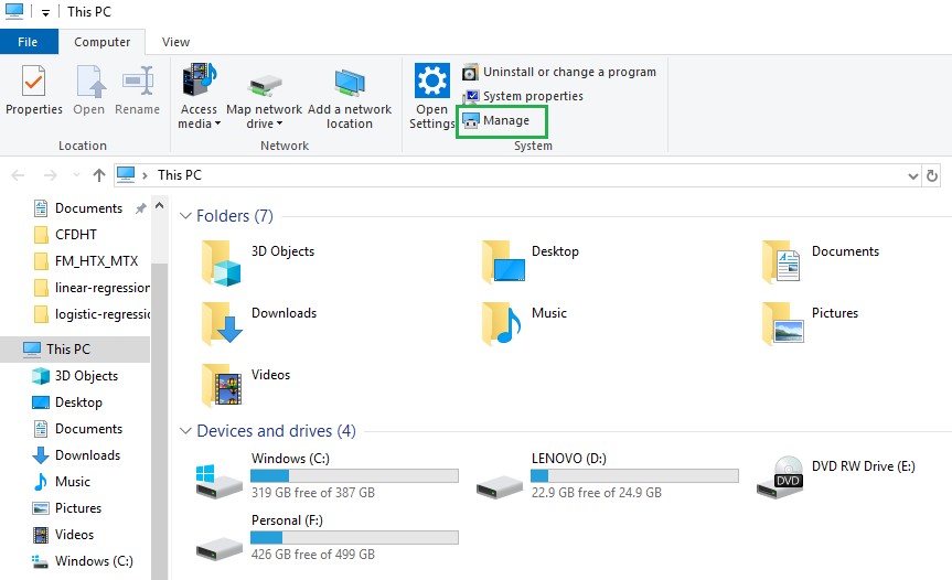
Starting FLUENT in batch mode: On Windows, the Ansys installer sets the environment variable. For instance, the Ansys 2025 R2 installer sets the AWP_ROOT252 environment variable to point to "C:\Program Files\ANSYS Inc\v252" if default installation location is selected. echo %AWP_ROOT232% can be used in a Batch file.
Linux:| fluent | 3d | -g | -i | batch.jou | -tN | -driver | opengl | -rx | 19.2 | -mpi=hp | -cnf=hosts.txt | >& | batch.out |
| 2d | -gr | -t8 | x11 | 19.1 | intel | ||||||||
| 2ddp | -gu | -t32 | null | 19.0 | ms | ||||||||
| 3ddp | -t96 | mpich2 |
Starting FLUENT in batch mode in Windows
@echo off
SET ANSYS_INSTALL_DIR="C:\Program Files\ANSYS Inc\v232"
SET WORKING_DIR="E:\Projects"
"%ANSYS_INSTALL_DIR%\fluent\ntbin\win64\fluent.exe" 3ddp -g -t4 -wait -meshing -i %WORKING_DIR%\geo_mesh.jou
"%ANSYS_INSTALL_DIR%\fluent\ntbin\win64\fluent.exe" 3ddp -g -t4 -wait -i %WORKING_DIR%\setup_run.jou
| fluent | 3d | -g | -i | batch.jou | -tN | -driver | opengl | -rx | 19.2 | -mpi=hp | -cnf=hosts.txt | -wait |
| 2d | -gr | -t8 | x11 | 19.1 | intel | -hidden | ||||||
| 2ddp | -gu | -t32 | null | 19.0 | ms | |||||||
| 3ddp | -t96 | mpich2 |
- -g indicates that the program (Cortex) is to be run without the GUI and graphics (Linux) or without graphics and with GUI minimized in the taskbar (Windows).
- -gr will run Cortex without graphics. This option can be used in conjunction with the -i option to run a job in background mode.
- -gu will run Cortex without the GUI but with the graphics window(s). (On Windows: it will run FLUENT keeping the window minimized that is the GUI will be available)
- -i reads the specified journal file say batch.jou
- -tN where N = number of processors = 2, 3, 4, ... 8, ... 32... -tmN: number of nodes for meshing, note there should be no space between t and N
- -driver allows to specify the graphics driver to be used in the solver session
- -gu -driver null allow the generation and export of graphics files from FLUENT simulation run in batch mode
- -aas: start FLUENT in server mode
- -command="TUI-Command" - tun TUI-Command on start-up
- -nm: do not display mesh after reading
- -post: run post-processing executable only
- -rREL: use release number REL
- -cnf=hosts.txt is the file with the names of the computational nodes (or the hosts)
- Fluent 19.0 onwards, the solver does not differentiate between a serial mode and a parallel mode. Now the serial mode is in fact the general parallel mode with just one parallel task, -t1 option explained above.
- For a ANSYS FLUENT session that is already in progress, the graphics window display can be disabled using the TUI command: display → set → rendering-options → driver → null
- For a ANSYS FLUENT session that is already in progress, to re-enable a graphics window display that had been previously disabled, use the TUI command: (close-all-open-windows); display → set → rendering-options → driver → opengl
Reference: doku.lrz.de/pages/viewpage.action?pageId=27394531
 WARNING: Rank:0 Machine mpp2-xxxxxxx has 37 % of RAM filled with file buffer caches.
This can cause potential performance issues. Please use -cflush flag to flush the cache.
(In case of any trouble with that, try the TUI/Scheme command '(flush-cache)'.)
In order to clear the buffer cache, add following lines at the beginning the journal file.
(rpsetvar 'cache-flush/target/reduce-by-mb 12288)
(flush-cache)
The number 12288 [Mb] = 12 x 1024 [kb] is the specification of the amount of system memory which cannot be flushed out due to boot image of Linux OS files in the memory of the diskless compute nodes. This means that on a compute node with 64 Gb, it tries to flush 64 [Gb] - 12.0 [Gb] = 52 [Gb] of memory. The value of 12288 also varies from cluster-to-cluster and may also change over the time.
The performance meter stores the wall clock time elapsed during a computation as well as message-passing statistics. Since the performance meter is always activated, the statistics can be printed after the computation is completed. To view the current statistics, use the Parallel/Timer/Usage menu item or TUI: paralle/timer/usage. There are many parallel statistics, few easy to decipher are:
- Average wall-clock time per iteration: it describes the average real (wall clock) time per iteration.
- Message count per iteration: it describes the number of messages sent between all processes per iteration. This is important with regard to communication latency especially on high-latency inter-connnects. A higher message count indicates that the parallel performance may be more adversely affected if a high-latency interconnect is being used. Ethernet has a higher latency than Myrinet or Infiniband. Thus, a high message count will more adversely affect performance with Ethernet than with Infiniband.
- Data transfer per iteration: this factor describes the amount of data communicated between processors/iteration. This is important with respect to interconnect bandwidth and is usually dependent on the algorithm being used and the problem being solved. This number generally increases with increases in problem size, number of partitions and physics complexity.
- LE wall-clock time per iteration: the factor that describes the time (wall-clock) spent doing linear equation (LE) solvers (i.e. multigrid).
- Total wall-clock time: it describes the total wall-clock time which can be used to gauge the parallel performance (speedup and efficiency) by comparing this quantity to that from the serial analysis. An approximation of parallel speed up may be found in the ratio of Total CPU time to Total wall clock time.
- The algebraic multigrid (AMG) solver for Fluent simulations is computationally intensive and in flow-only problems typically the coupled solver spends about 60~70% of run-time solving the linear system using AMG.
- On the other hand, segregated solver spends only 30~40% of run-time in AMG computation. One can find out AMG portion of a Fluent calculation (and therefore whether it is a good candidate for GPU deployment) by adding the command '/parallel/timer/usage' to the journal file for a CPU-only run.
- The information is reported towards the end of the output file after successful completion of calculations. Output message would look something like: "LE wall-clock time per iteration: 5.678 sec (67.8%)".
- Additionally, stiff matrices are difficult to solve and require more inner-loop iterations in the AMG solver.
- Add these TUI in scheme file: parallel/latency and parallel/bandwidth.
Activating GPU in FLUENT runs
GPGPU stands for General Purpose GPU. The available GPU can be check in FLUENT TUI suing scheme command: /parallel/gpgpu. The GPGPU can be turned on for specific equation solver by TUI: /solve /set /amg-option /amg-gpgpu-option. The options are k, ε, temperature and pressure-velocity coupling.Ansys Remote Solve Manager
Excerpts from User Guide: "Ansys Remote Solve Manager (RSM) provides the central framework for job submission to an established cluster or third-party Cloud. This enables you to access powerful compute resources when needed. To enable job submission to a cluster or Cloud portal, an administrator must create configurations in RSM. An RSM configuration contains information about the HPC resource where jobs are submitted (such as the name of the cluster submit host, or URL of the web portal), file transfer methods, and the queues that are available for job submission." The RSM is required for parametric studies where geometry is updated in ANSYS Discovery on local machine running on Windows OS, meshing/simulation runs are being made on remote Linux cluster and finally post-processing is done using CFD-Post within Workbench environment. A problem statement like "Run parametric design updates (involving geometry changes) where the FLUENT Meshing and the FLUENT solver is executed on Linux cluster and the geometry updates with ANSYS Discovery will be done on a window machine" will require RSM.
Alternatively, use telnet "hostname or IP address" "port number" such as telnet 10.21.34.55 9252. Telnet Client can be turned on using "Turn Windows features on or off" by the administrator. If only the blinking cursor is visible, then the port is open.
Every RSM installation has one predefined configuration named localhost. This configuration uses a basic Ansys RSM Cluster (ARC) to submit jobs to the local machine. This enables users to run certain types of local jobs or Mechanical background jobs right out of the box, without any special setup.
When you submit a job to RSM from Workbench for the first time, RSM will prompt you to specify credentials for accessing the HPC resource associated with the chosen RSM queue. RSM will validate and cache the credentials, and there will be no need to specify credentials again unless your password changes.
Since RSM requests, validates and caches your credentials when you first submit a job to RSM, it is generally unnecessary to manually create user accounts in RSM. If you would prefer to cache your password in advance of submitting jobs to RSM (for example, if you want to run a Workbench job in batch mode), you can add an account in RSM that contains the credentials necessary to access the HPC resource, and apply the account to the RSM configuration that is associated with that HPC resource. The password cannot contain special characters, or characters with special marks such as accents.
C:\Windows\Temp and %TEMP% folders contain logs file generated by RSM Launcher Service and RSM UserProxy process respectively.A user proxy process is created for every user who submits a job to RSM. Each user proxy process will use a separate port chosen by RSM. By default, RSM will randomly select any port that is free.
Error: "LauncherService at machine: 9242 not reached" > Ensure that the launcher service is running > If a local firewall is on, add port 9242 to the Exceptions List for the launcher service (Ans.Rsm.Launcher.exe) > Allow a ping through the firewall (Echo Request - ICMPv4-In) > Enable "File and Printer Sharing" in firewall rules.


Batch Runs: CFX
cfx5solve -batch -double -parallel -def input.def  \
-n 32 -start-method "Intel MPI Distributed Parallel"  \
-par-dist "$HOSTLIST" -continue-from-file input.res
The flag -double starts double precision versions of Partitioner, Interpolator and Solver. The -par-dist option is used to specify the list of names of nodes (hosts) and corresponding numbers of cores (tasks) of each node applied for performing numerical simulations (e.g. host1*N1, host2*N2). The list of names of computational nodes is generated automatically and is stored in the HOSTLIST variable. This is done by job scheduler such as PBS, SLURM, Univa Grid Engine. To stop a run on cluster: Suppose a run is called Project_001, there will be a temporary directory called Project_001.dir in the run work directory. The command "touch Project_001.dir/stp" shall create a empty stop file named 'stp'. Alternatively, create the empty file named 'stp' on host machine and upload in 'Project_001.dir' folder on cluster.
Batch Runs: ICEPAK
The parallel runs can be made in multiple ways: parallel run on a host, parallel run on a network known as "Network Parallel" in ICEPAK and parallel runs on a job-scheduler.- Create an ICEPAK session and read project named proj_name.prj: icepak proj_name.prj
- Create ICEPAK session and read a compressed (archived) project in tzr format: icepak -unpack proj_name.tzr
- Set auto-save interval for transient runs: "Solution Save Interval" specifies how often the intermediate results file be saved. Every tenth time-step is saved by default. *.fdat file is saved as specified interval and *.dat file is saved only at the end of the solution
- Set auto-save interval for steady state runs: Solve -> 'Results' tab -> "Solver Data" section -> "Auto-save Interval" -> Specify number of iterations
- Solve -> 'Advanced' tab -> "Reuse existing meshes", "Merge zones when possible"
- Create Restart solution files: Solve -> 'Results' tab -> "Solver Data" section -> Write interpolated restart data file or Write full restart file: interpolate data when "Geometry and mesh are different", Full data: use when geometry and mesh are identical (exactly same)
- Create script file for Batch Processing: Solve -> 'Advanced' tab -> "Submission options" section -> Script file: specify the file name -> "Solver preprocessing" section -> "Don't start solver: turn ON -> Click "Start Solution" button to generate the script file.
Batch Mode: ANSYS Workbench
To run Workbench in batch or interactive mode and execute a Python script via Windows/Linux shell: installPath/RunWB2.exe -B -R path/Script.py ---The Installation Path is the absolute path to the Workbench executable. -B refers to batch mode, -R is to run specified script file. Linux: path/runwb2 -B -R journal.wbjn > logWB.txt to run a Workbench journal, here 'path' is the installation folder. Typically, WB journal would be required to [1]read in the project, [2]generate the mesh, and [3]save the project.In Workbench, Python scripts can be executed by: "File > Scripting > Run Script File" and choosing a *.py file. Alternatively, command(s) can be executed by using "File > Scripting > Open Command Window" and executing the intended commands.
Batch Mode: FEA programs
LS-DYNA is a general-purpose finite element program capable of simulating complex problems in automotive, aerospace, construction, military, manufacturing, and bioengineering industries. The code uses highly non-linear, transient dynamic finite element analysis using explicit time integration for analyzing high speed, short duration events where inertial forces are important. Typical uses include automotive crash, explosions, manufacturing... Large LS-DYNA models are computationally intensive both from run-time and storage point of view.Log files
CFX creates a log file *.out | LS-DYNA writes a file named ls-dyna.log | Abaqus generates several files some of which (such as *.lck) exist only while ABAQUS is executing and are deleted when a run completes whereas other files contain analysis, post-processing, and translation results (such as *.abq, *.fil, *.odb) and are retained for use by other analysis options, restarting, or post-processing.License Manager: LMTOOLS
Most of the CFD programs be it ANSYS FLUENT or STAR-CCM+ use LMTools to manage the licenses at their customers. The executable utility is installed in the same folder where main program such as ANSYS FLUENT is installed. The syntax to use LMSTAT is: lmstat [-a] [-c license_file_list] [-f [feature]] [-i [feature]] [-s[server]] [-S [vendor]] [-t timeout_value]. The purpose of each option is:- -a: Displays all information
- -c license_files: Uses the specified license files
- -f [feature]: Displays 'users' of feature. If feature is not specified, all features are displayed
- -i [feature]: Displays information from the feature definition line for the specified feature, or all features if feature is not specified
- -s [server]: Displays status of all license files listed in $VENDOR_LICENSE_FILE or $LM_LICENSE_FILE on server, or on all servers if server is not specified
- -S [vendor]: Lists all users of vendor’s features
- -t timeout_value: Sets connection timeout to timeout_value which limits the amount of time 'lmstat' spends attempting to connect to server.
"C:\Program Files\ANSYS Inc\Shared Files\licensing\winx64\lmutil" lmstat -a -c 1055@server_name: This will produce a list of all licenses and any current checkouts. The following example checks the information on the feature cfd_base "C:\Program Files\ANSYS Inc\Shared Files\licensing\winx64\lmutil" lmstat -a -f cfd_base -c 1055@server_name. On Linux, path would be: /ansys_inc/shared_files/licensing/linx64/lmutil lmstat. Other feature names are: fluent_meshing, cfd_preppost, cfd_preppost_pro, anshpc_pack, acfx_pre, cfd_solver_level1, cfd_solver_level2
Finding Names of Feature: to use -f option, one need to know the exact names of features. This can be found in license.dat file or check the output from -a options. lmutil.exe lmstat -s licServers -f "feature_name"
For scripting and partial automation of pre-processing, solver and post-processing activities, refer to this section of scripting page.
For dealing with file handling in Linux and Windows, refer to short summary of shell scripting.
Material Definition in Text File
Material properties in OpenFOAM is always defined in a text file. Similarly, FLUENT can read material in *.scm file as per following format. The extension 'scm' stands for SCHEME file.(
(air
fluid
(chemical-formula . #f)
(density (constant . 1.225)
(premixed-combustion 1.225 300))
(specific-heat (constant . 1006.43))
(thermal-conductivity (constant . 0.0242)
(polynomial -3.933E-04 1.018E-04 -4.857E-08 1.521E-11)
)
(viscosity (constant . 1.7894e-05)
(sutherland 1.7894e-05 273.11 110.56)
(power-law 1.7894e-05 273.11 0.666)
)
(molecular-weight (constant . 28.966))
)
(aluminum
solid
(chemical-formula . al)
(density (constant . 2719))
(specific-heat (constant . 871))
(thermal-conductivity (constant . 202.4))
(formation-entropy (constant . 164448.08))
)
)
When FLUENT opens, it auto executes the .fluent file in the: home directory of Linux users, C:\ directory of Windows machines. A .fluent file can contain any number of scheme file names to load. Unless full path is specified for each scheme file in .fluent file, FLUENT tries to
locate the scheme files from the working directory. Sample .fluent file is described below. #t is to set boolean flags TRUE and #f is to set it FALSE.
(load "plot.scm")
(let ((old-rc client-read-case))
 (set! client-read-case
  (lambda args
  (apply old-rc args)
  (if (cx-gui?)
   (begin
    ;Do the customization here
     (rpsetvar 'residuals/plot? #t)
     (rpsetvar 'residuals/settings '(
      (continuity #t 0 #f 0.00001)
      (x-velocity #t 0 #f 0.00001)
      (y-velocity #t 0 #f 0.00001)
      (z-velocity #t 0 #f 0.00001)
      (energy #t 0 #f 1e-06)
      (k #t 0 #f 0.00001)
      (epsilon #t 0 #f 0.00001)
      )
     )
     (rpsetvar 'mom/relax 0.4)
     (rpsetvar 'pressure/relax 0.5)
     (rpsetvar 'realizable-epsilon? #t)
     (cxsetvar 'vector/style "arrow")
    )
   )
  )
 )
)
Troubleshooting Convergence in FLUENT
For all iterative solvers, the solution is quickly and smoothly achieved if the initial guess is closer to expected value. This is not always possible in CFD simulations with mean flow direction not aligned to coordinate system. The standard approach to handle such situation is as follows:Step-01: Start with laminar or turbulent flows with first order (Upwind) discretization schemes. Use incompressible fluid properties. Turn off energy equation - that is temperature field shall not be solved. Run for 500 iterations.
Step-02: While keeping incompressible fluid properties, turn ON energy equation - that is temperature field shall be solved. Run for 1000 iterations.
Step-03: While keeping incompressible fluid properties, energy equation ON, change discretization scheme for momentum to second order [Central Difference Scheme]. Run for 500 iterations.
Step-04: Change fluid properties to ideal gas or incompressible-ideal-gas as the case may be.
Step-05: Optionally, change the discretization scheme for turbulence parameters (k, ε ω) to second order.
All these steps can be build into a single journal script while making batch runs and there is not need to make separate runs for each step mentioned above.Error message: Divergence detected in AMG solver: temperature
- Reduce explict-relaxation in TUI:
- (rpsetvar 'temperature/explicit-relax? #f)
- (rpsetvar 'explicit-relaxation? #t)
- (rpsetvar 'temperature/explicit-relax 0.9) - By default, explicit-relax is set to 1.0.
- Turn OFF secondary gradient on all the cells: (rpsetvar 'temperature/secondary-gradient? #f). By default, this is #t (true). To obtain the value, type: (rpgetvar 'temperature/secondary-gradient?) which will return either #t or #f.
- Turn OFF secondary gradient in shell conduction zones: (rpsetvar 'temperature/shell-secondary-gradient? #f)
Note: 'secondary-gradient' mentioned above is not the higher-order derivatives, but relates to additional correction term used to compute diffusive heat flux across cell faces particularly important for non-orthogonal meshes. Global deactivation of secondary gradient should be employed as a last resort keeping in mind inaccuracies it brings. Improving mesh quality / refinement should be considered prior to this option.
Sometimes you may get unrealistic temperature and pressure values. Check that velocity field has reasonable values. This may be due to incorrect mass flow rate or incorrect scaling of the mesh or mesh with aspect ratio > 200 or cells with orthogonality > 0.98.S2S Fiew Factor Reading Error: While reading view factors on a HPC cluster, following 'fatal' error occurs:
Error reading case file
Error: File pointer could not be allocated for testCase.s2s.h5.
Solution: Read only the case file through journal, generate s2s view factor file through TUI command and proceed with other operations.
Improve Heat Balance Rate in S2S Radiation Model: Set the "Residual Convergence Criteria" to a value lower than default which is 0.001, increase number radiation solver iterations by changing "Maximum Number of Radiation Iterations" from default value of 5 to a higher value say 25 or 50. When convergence problems with radiation do occur, investigate the radiation solver convergence by turning off the 'flow' and 'turbulence' equations temporarily. Once the issues with S2S model alone are resolved, activate Flow and Turbulence again to proceed to the final solutions.
Domain containing higher fraction of volume with dead zones or creeping flow conditions: While dealing with creeping flow or a simulation with large fraction of computational domain with nearly zero velocity, coupled solvers tend to be robust than segregated solvers.
Memory Related Issues: Following error might be due to insufficient memory required for solver, including a faulty computational node while parallel processing.
=== Message from the Cortex Process ===Fatal error in one of the compute process
ANSYS Workbench
ANSYS has an option to maintain the geometry, mesh, solver and post-processing application inside a common project structure defined as Analysis Systems and Component Systems. Analysis system is a 'Set' of all necessary Component Systems while the later comprise of stand-alone editors to build the projects. The component "Fluid Flow (Fluent)" uses ANSYS Meshing and "Fluid Flow (Fluent with Fluent Meshing)" uses Fluent mesher as the mesh generation tool. Bidirectional associativity between SCDM and native CAD (Inventor, Creo...) requires additional add-ons.Change default start-up folder path (launch directory): this method is same for any other program in Windows. Search Workbench in the start menu, right click and select open file location, right click on Workbench executable and select Properties, Change the "Start in" path from "%HOMEDRIVE%%HOMEPATH%" to any other location and click OK. It may ask for an administrator password. On Windows, the default location of Workbench Log Files is %TEMP%\Workbench-Logs.
ANSYS Workbench scripting guide summarizes class, methods and properties. GetUserPathRoot() is a method which return WB root path as string. SetUserPathRoot() can be used to change this value for the current session only. IsProjectUpToDate() method returns True or False depending upon status of the project. GetAllSystems[0] .Components[0] returns "/Schematic/Component: Geometry" and GetAllSystems[0] .Components[0] .DataContainer returns 'Geometry'. GetAllSystems[0].Physics returns ['Fluids'], GetAllSystems[0] .Solver returns ['FLUENT'] and GetAllSystems[0] .SystemType returns "Fluid Flow (Fluent with Fluent Meshing)". Similarly,- GetAllSystems()[0] .Components[0] .DataContainer .GetFiles() - get the file names
- GetAllSystems()[0] .GetContainer(ComponentName = "Geometry") .GetAllParameters()[1].Name = P1, the name of second parameter.
- Parameters.GetDesignPoint(Name="0") .HasValidRetainedData = True or False as the case may be
- Parameters.GetDesignPoint(Name="0") .StateOfParameters = 'NeverSolved'
Close without Saving: All applications started from Workbench cannot be exited until they are saved. However, the file itself is not changed until the Workbench project is saved, exit Workbench without saving it and return to the last saved state. All operations on Workbench and applications started in Workbench save their contents to a temporary folder (.Project name.backup) and files in the original project folder are not changed until the project is saved.
To monitor solutions: Right click on the 'Solution' cells and select "Show Solution Monitoring". Error Message: "Model information is incompatible with incoming mesh" - right click on Setup cell, select 'Reset' and then update the project. Alternatively, right click on the Project type cell (such as "Fluid Flow (Fluent with Fluent Mesher") and select Clear Generated Data. If the case set-up does not have number of iterations defined, the update of solution cell shall throw error: "Setup needs non zero number of Iterations or Timesteps to be marked as UpToDate."
If the stop/interrupt icon in progress bar is missing, rename or delete the folder under %appdata%Ansys/v212/ folder. This will reset the Workbench settings. If a run or update is in progress, do not open any file in dpN folder which is continuously updated (such as *.trn or *.out files), the operation may get stuck and the interrupt icon may also disappear. Copy the monitor or output file and save it to other location to view the content, required specially when "Solution Monitoring" for 'Solution' cell is turned off.
It is not possible to switch from meshing mode to solution mode with a different number of processes on Windows, so in case it is needed to run the solver with higher number of processes a new (solver) session is required. Similarly, if there is any changes in Geometry cell of the project (such as creation of new Named Selections) which require manual update, the Mesh cell needs to be opened in GUI mode and meshing workflow needs to be updated for later batch updates.
Folder Structure
| Case_1_files/ (Project Name = Case_1.wbpj) | ||||
| dp0/ | FFF/ | DM/ | FFF.scdoc | |
| Fluent/ | ||||
| FFF_workflow_files/ | ||||
| Workflow/ | ||||
| *.out (monitor files) | ||||
| FFF.ip | ||||
| FFF.msh | ||||
| FFF-1.cas.h5 | ||||
| Post/ | ||||
| dpall/ | global/ | ACT/ | extension/ | |
| progress_files/ | dp0/ | FFF/ | ||
| session_files/ | *.wbjn | - | - | |
| user_files/ | DesignPointLog.csv | - | - | |
The Files pane (access through Files item in the View menu) shows a list of all files associated with the project. It enables users to see the name and type of file, the IDs of the cells the file is associated with, the size of the file, the location of the file, and other information.
The files in dpN (dp0, dp1...) folders are used by Workbench to save only those files which are updated within the Project. It is recommended not to save any file that is not updated within Workbench in these folders else it will get delete during next update. In many cases when standalone sessions of Fluent are used to save case / data files in these folders (e.g. for re-run or transient cases), Workbench will delete these files when the project is updated later.
Using script:- GetProjectFile(): This returns the absolute path of currently opened *.wbpj file
- GetProjectDirectory(): returns the full path of the folder from where *.wbpj file is loaded
- GetUserFileDirectory(): get location of user_files/ directory, absolute path with '\' escaped with '\\'
- os.path.join() can be used to create full path for any files to be used to save, open, import and export.
- GeometryFilePath: The location of file currently assigned to geometry component. DesignModeler process this file when started through Edit command.
Icons and their Meanings
![]()
In Workbench, multiple 'Geometry' components cannot be used to create a assembly. For example, the Rotor, Stator and Enclosure cannot be stored in separate 'Geometry' components and all linked to a common 'Geometry' component.
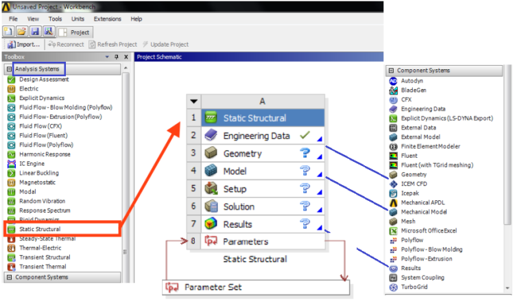
- cfx_sys = GetTemplate(TemplateName = "Fluid Flow", Solver = "CFX").CreateSystem()
- fluent = GetTemplate(TemplateName = "Fluid Flow") - Fluent project with ANSYS Meshing
- fluent = GetTemplate(TemplateName = "Fluid Flow with Fluent Meshing") - Fluent project with Fluent Meshing
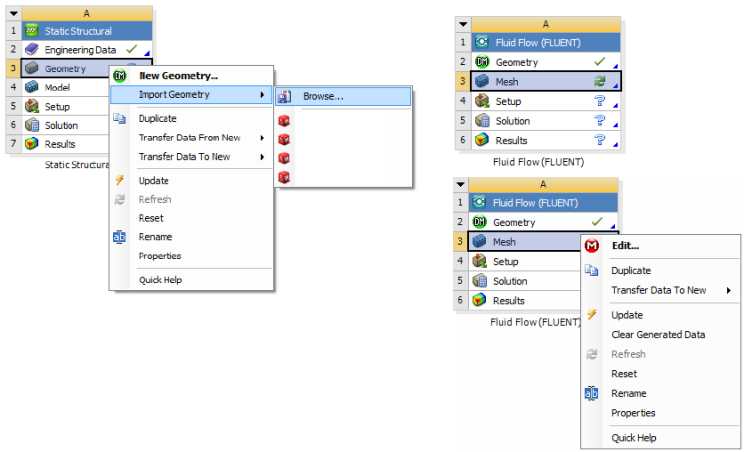
- cfx_comp = GetTemplate(TemplateName = "CFX").CreateSystem()
- flu_comp = GetTemplate(TemplateName = "FLUENT")
- tgd_comp = GetTemplate(TemplateName = "FLTG")
- geo_comp = GetTemplate(TemplateName = "Geometry")
- dsc_comp = GetTemplate(TemplateName = "Discovery")
- msh_comp = GetTemplate(TemplateName = "Meshing")
- res_comp = GetTemplate(TemplateName = "Results")


Found some missing and new zones in the mesh. To make mesh compatible with settings, please visit "Match Zone Names" panel. (Mesh > Recorded Mesh Operations > Edit Incoming Zones... > Match Zone Names...). This occurs when in a Fluent system, Geometry and Mesh components are lined to a Fluent case and later something is changed in mesh. This requires the link between the Fluent case file and the mesh to be updated manually - that is open the Setup component in GUI mode, let the case get updated and save the case file.
Run Workbench using Python Script
import subprocess as sp
wb = r"C:\\Program Files\\ANSYS Inc\\v222\\Framework\\bin\\Win64\\runwb2.exe -I -R E:\Projects\Script.py"
sp.Popen(wb)
-E option can be used to pass arguments to *.wbjn script: runwb2.exe -E "var1=20" -E "var2=50" -R wb_script.wbjn where var1 and var2 are defined in *.wbjn file.
import os
sys = GetAllSystems()[0].GetContainer(ComponentName = "Setup")
sys_type = sys.GetMechanicalSystemType()
sys_name = sys.Name

# Clear Generated Data, multiple systems can be specified
CleanSystem(Systems=[sys])

# Get the system name and change its display name (no index available)
base_sys = GetSystem(Name = "FFF") # GetSystem(Name = "FLU")
#base_sys.Type = System, base_sys.Name = FFF, FFF 1, FFF 2 ....
if "FFF" in base_sys.Name:
  base_sys.DisplayText = "DP_001"

n_start = 2  # Assumes one baseline system is already created
n_end   = 5
for i in range(n_start, n_end+1):  # range function excludes last value
  new_fluent_sys = base_sys.Duplicate()
  new_fluent_sys.DisplayText = f"DP_{i: :03d}"

#GetComponentState(GetAllSystems()[0].GetComponent("Solution")).State
#cell_state = GetCellDisplayState(comp)
#print(cell_state.State)

#check if System in WB contains a particular component say 'Results'
sys =  GetAllSystems()[0]
def checkComponent(sys, comp_name):
  for comp in sys.Components:
    if comp_name in (comp.Name):
      return True
# Usage: check_comp = checkComponent(sys, "Results")

def needsUpdate(comp):
  if GetComponentState(comp).State != "UpToDate":
    return True

geo_cell = base_sys.GetContainer(ComponentName="Geometry")
#geo_cell.SetFile(FilePath = r"E:/Projects/Geom.scdoc")

geo_comp = base_sys.GetComponent(Name="Geometry")
geo_comp.Refresh()
if geo_cell is not None:
  if needsUpdate(geo_comp):
    geo_cell.Update()
else:
  print(f"No Geometry cell found in system {i}: {base_sys.DisplayText}")
The SpaceClaim and Discovery applications are not supported on Linux as in version 2024. Hence, any script to use Linux cluster for geometrical operations shall not work. The CAD geometry needs to be exported in *.pmdb (Parametric Model Database) format. Workbench.Fluent .ExportPMDB(r "E:\Projects\Case-1.pmdb"). To run Python file through a command line window in Workbench, ACT console can be used with print statements to check the progress. Use following method to save the SCDM file in *.pmdb format, note the geometry files are saved as FFF.scdoc in dpN folder within Workbench. Commands need to be send line by line and not as a group of multiple statements.
geom_scdm = fff.GetContainer(ComponentName = "Geometry")
# SpaceClaim and Discovery require GUI mode to create/manipulate geometry
geom_scdm.Edit(IsSpaceClaimGeometry = True, Interactive = True)

# Following does not save the file in PMDB format neither reports any error
geom_scdm.SendCommand("Workbench.Fluent.ExportPMDB('FFF.pmdb')")
'''
# Following 2 statements does not create PMDB file neither reports any error
cmd = """Workbench.Fluent.ExportPMDB(FFF.pmdb)"""
geom_scdm.SendCommand(Language = "Python", Command = cmd)

# Following single line script run through *.wbjn file does not save PMDB file
geom_scdm.RunScript(ScriptFile = "scdm.py", useAsMacro = "False")
# Here, content of the file scdm.py is: Workbench.Fluent.ExportPMDB('FFF.pmdb')
'''
geom_scdm.Exit()
The export command exports geometry data in the running geometry editor to the location specified in its FilePath argument. The export file CAD format is deduced from the extension of FilePath.
geom_scdm.Export(FilePath = AbsUserPathName("FFF.step"))
Alternatively, read commands stored in a file as described here. Block of commands can be created between """ ... """ and even variables can be used inside the block as described below. Though they need to be sent one by one using SendCommand:
cmd = """
Reset()
import clr
clr.AddReference("SpaceClaim.Api.V232")
from SpaceClaim.Api.V223 import *
Lx = 100
Ly = 200
Lz = 500
sec_plane = Plane.PlaneZX
gen_plane = ViewHelper.SetSketchPlane(sec_plane, Info1)
...
P1 = Point.Create(MM(%s), MM(%s), MM(%s))
"""%(Lx, Ly, Lz)

for line in cmd.splitlines():
  geom_scdm.SendCommand(Language="Python", Command=line)
# Loop over all systems in the schematic
for system in GetAllSystems():
  # Edit model components in batch mode
  system.Refresh()

  mesh_cell = system.GetContainer(ComponentName="Mesh")
  mesh_cell.Update()
  #mesh_cell.Edit(Interactive=False)

  setup_comp = system.GetComponent(Name="Setup")
  setup_comp.Refresh()
  #
  setup = system.GetContainer(ComponentName="Setup")
  #
  #setup.Edit(Interactive=False))
  #setup.SendCommand(Command='/file/read-journal "setUp.jou"')
  setup.Update()
  #
  solution_cell = system.GetContainer(ComponentName="Solution")
  solution_cell.Update()

# To update all components in a single statement
results_comp = system.GetComponent(Name="Results")
results_comp.Update(AllDependencies=True)

Save(OverWrite=True)
To read Python Commands from a File
script_file = open(r"E:\Projects\script.py", "r")
script_cmd = script_file.read()
script_file.close()
setup = system.GetContainer(ComponentName = "Setup")
setup.Edit(Interactive=False)
setup.SendCommand(Language = 'Python', Command = script_cmd)

# \ and quotes (") needs to be escaped when specifying directly as arguments
setup.SendCommand(Command="/file/read-journal \"E:\\Projects\\script.jou\"")
# just the TUI: FLUENT internal Scheme commands may not work properly when
# called directly using the SendCommand method
setup.SendCommand(Command="/define/models/viscous kw-sst y")
setup.SendCommand("define model energy yes")
setup.SendCommand(Command="(cx-gui-do cx-activate-item \"MenuBar*FileMenu*Close FLUENT\")")
Import Geometry in SpaceClaim from Project Schematic: reference discuss.ansys.com
fff = GetTemplate(TemplateName="Fluid Flow (Fluent)")
#ssa = GetTemplate(TemplateName="Static Structural", Solver="ANSYS").CreateSystem()
sys = fff.CreateSystem() # GetAllSystems()[0]

CAD_file = r"E:\Project\Fluid.igs"
geo = sys.GetContainer(ComponentName="Geometry")
geo.Edit(IsSpaceClaimGeometry=True)

def importFile(file_name):
  geo_import ="""DocumentInsert.Execute(r""" + """ + file_name + """ +""")"""
  return geo_import
cmd_geo_import = importFile(CAD_file)
geo.SendCommand(Language="Python", Command=cmd_geo_import)
Helper function to write parameters to a log file. Parameters.SetBaseDesignPoint(DesignPoint = DP1) can be used to set any specific design point as 'Current'. Here, dp1 = Parameters.GetDesignPoint(Name = "1"). To change the value of a parameter: p1_x = Parameters.GetParameter(Name="P13"), dp1.SetParameterExpression(Parameter = p1_x, Expression = "0.05 [in]")
def writeParams(log_file):
  for param in Parameters.GetAllParameters():
    par_str = " " + param.Name + ": " + param.DisplayText + " = " + param.Value.ToString()
    log_file.write(par_str + "\n")
    log_file.flush()
param.ValueQuantityName, param.Value.Unit, dp1.GetParameterValue(param).Value are used to access parameter value type, unit and the value. Two lists can be declare using one statement: list_1, list_2 = ([] for i in range(2)).
Walk through the systems and components, to find any that are using the file. This method provides detailed information about systems, components and file references. It is also a useful example of general System and Component navigation.
for system in GetAllSystems():
  for component in system.Components:
    container = component.DataContainer
    # Loop over file data references associated with container for the component
    for comp_file in container.GetFiles():
      if comp_file.FileName.find(target_file) > -1:
        log_file.write("--\n")
        sys_str = "Target file found in component %s of system %s in %s.\n"
        file_str = "%s, Size %s bytes, Modified %s\n"
        log_file.write(sys_str % (component.DisplayText, system.DisplayText, proj_file))
        log_file.write(file_str % (comp_file.Location, comp_file.Size, comp_file.LastModifiedTime))
        logFile.flush()
  log_file.close()
When using Update All Design Points, turn on the Retain option (click the checkbox under Retain column in the table of design points). This will save the files for the completed design points. This option is required to set any any design point as Current. However the main Workbench project cannot be saved using any direct option, scripting can be used for this.
When you manually update a design point to current design, the status of earlier design points shall change to "Update Required" even though nothing has change for each row item. The Workbench treats the analysis system as altered even if a post-level item is added to the project. Select the required design points, right click and choose "Export Selected Design Points" which writes a new project containing only those design points. This project can be opened in a new Workbench session.
When using Update All Design Points, the update of Mesh cell gets stuck, it may point to creation of invalid geometry such as deletion of a face or named selection or reference edge / face. If geometry is correct, turn off "Solution Monitoring" in properties panel of the 'Solution' cell. Also check which option for initialization under properties panel of 'Solution' cell works for that particular case: Program Controlled or Solver Controlled. Using "Run Script File..." command does not show the progress.
Update Design Points using Script: works only if the mesh is not already generated. If the selected design point is already 'Current', SetBaseDesignPoint() shall not work. Use dpc = Parameters.GetActiveDesignPoint() to access currently active design point. dpc.DisplayText prints "DP 3" is fourth design point is active. dpc.Name shall print '3'. When running such script, update the preferences in FLUENT or issue TUI "preferences general startup-message color-theme-change-message no" to prevent the pop-up windows when FLUENT session starts.
dp_num_start = 1  # Note zero-based index. 1 = second DP
dp_num_final = 4
system = GetSystem(Name="FFF")
setup = system.GetContainer(ComponentName="Setup")
launcher = setup.GetFluentLauncherSettings()
launcher.ShowLauncher = False
launcher.DisplayMesh  = False

# Loop overall design points in the rage dp_num_start and dp_num_final
for i in range(dp_num_start, dp_num_final+1):  # range method excludes 'stop' number

  # Increment to next design point
  dp_i = Parameters.GetDesignPoint(Name=repr(i))
  dp_current = Parameters.GetActiveDesignPoint().Name
  if dp_current != str(i):
    Parameters.SetBaseDesignPoint(dp_i)
  if dp_i.Retained == False:
    dp_i.Retained = True

  geom_comp_i = system.GetComponent(Name="Geometry")
  geom_comp_i.Update(AllDependencies=True)

  # Open fluent meshing, generate mesh, and close
  mesh_i = system.GetContainer(ComponentName="Mesh")
  Fluent.Edit(Container=mesh_i)
  setup.SendComman(Command='(cx-gui-do cx-activate-tab-index "NavigationPane.Frame1(TreeTab)" 0)
  (cx-gui-do cx-activate-tab-index "NavigationPane.Frame1(TreeTab)" 1)')
  mesh_comp_i = system.GetComponent(Name="Mesh")
  mesh_comp_i.Refresh()

  setup.SendComman(Command='/file/set-tui-version "24.2"(cx-gui-do cx-activate-tab-index
  "NavigationPane.Frame1(TreeTab)" 0)')
  setup.SendComman(Command="(newline)")
  setup.SendCommand(Command="(%py-exec \"workflow.TaskObject['Generate the Volume Mesh']
    .ExecuteUpstreamNonExecutedAndThisTask()\")")
  setup.SendComman(Command="(newline)")
  setup.SendCommand(Command='(cx-gui-do cx-activate-item "MenuBar*FileMenu*Close Fluent")')

  # Update 'Setup' component
  setup_comp_i = system.GetComponent(Name="Setup")
  setup_comp_i.Refresh()
  setup_comp_i.Update(AllDependencies=True)
  #setup.Edit()
  #setup.SendCommand(Command='(cx-gui-do cx-activate-item "MenuBar*FileMenu*Close Fluent")')

  # Update 'Solution' component
  sol_comp_i = system.GetComponent(Name="Solution")
  sol_comp_i.Refresh()
  sol_comp_i.Update(AllDependencies=True)
Update All Design Points
dp_list = Parameters.GetAllDesignPoints()
for i in range(len(dp_list)):
  dp_i = Parameters.GetDesignPoint(str(i))
  UpdateAllDesignPoints(DesignPoints=[dp_i])
  Save(Overwrite= True)
Create Design Points using Script
Export up-to-date parameter values of all the design points of the project. Parameters.ExportAllDesignPointsData(FileName = "DPs.csv")Prerequisite: project already has parameters defined, a CSV file with a header row matching the parameter names (or parameter display names) created. Run script within Workbench Scripting Console accessed through Tools > Scripting > Scripting Console.
import csv
from System import Array
from System.Collections.Generic import List

# Get geometrical parameters and those defined in CSV file
geo_container = system.GetContainer(ComponentName="Geometry")
geo_params = geo_container.GetAllParameters()

csv_file = r"C:\Projects\DPs.csv"
with open(csv_file, 'r') as csvfile:
  csv_reader = csv.DictReader(csvfile)
  csv_data = [row for row in csv_reader]

# Get names of the parameters from the project and check with names in CSV file
project_params = {p.DisplayText: p for p in geo_params}
csv_params = csv_reader.fieldnames
missing_params = [p for p in csv_params if p not in project_params]
if missing_params:
  raise ValueError("CSV parameters not found in project: " + ", ".join(missing_params))

# Add design points
for row in csv_data:
  newDP = Parameters.CreateDesignPoint() # dp = Parameters.GetDesignPoint("0")
  for param_name in csv_params:
    param = project_params[param_name]
    value = float(row[param_name])
    newDP.SetParameterExpression(param, str(value))

# Copy a design point multiple times
n_dp_copies = 5
source_dp = 1

dp_source = GetDesignPoint(source_dp)
params_dp = dp_source.GetInputParameters()
for i in range(n_dp_copies):
  new_dp = CreateDesignPoint()
  for par in params_dp:
    par_val = dp_source.GetInputValue(par)
    new_dp.SetInputValue(par, par_val)
'''
Manual Method (Parameter names and units must match exactly when importing)
1.
Export the current Design Points by right-click on top left corner or left
column of "Table of Design Points" > Export Table to CSV
2.
Edit CSV file by copying the desired row multiple times. Modify the input
values as needed.
3.
Import modified CSV (same as exporting CSV file) use Import Table from CSV.
'''
# Run All Design Points Automatically
param_manager.EvaluateAllDesignPoints()
Script to run at the project level that creates a Fluent component system, and then opens SpaceClaim to import a geometry file
fff = GetTemplate(TemplateName="FFF")
system = fff.CreateSystem()

CAD_file = r"C:\Users\Project\Geom.igs"
geom = system.GetContainer(ComponentName="Geometry")
geom.Edit(IsSpaceClaimGeometry=True)

def importFile(file_name):
  cmd="""DocumentInsert.Execute(r""" + """ + file_name + """ +""")"""
  return cmd
cmd = importFile(CAD_file)
geom.SendCommand(Language="Python", Command=cmd)
Sample Template for DOE: DP = Design Point
Create a worksheet named 'DOE-Parameters' containing following information.
| Variable Name | Description | Reference Object | Reference Direction | Level Low | Level High | Mean or Baseline |
| VP01 | Fin Height | Mounting Face | +X | 10 | 20 | 16 |
| VP02 | Fin Length | Front Face | +Y | 50 | 75 | 60 |
| ... | ||||||
| VP05 | Fin Pitch | Inner Faces | +Z | 2.0 | 5.0 | 2.5 |
| ... |
| VP01 | VP02 | ... | VP05_1 | VP05_2 | ... | VP05_8 | ... | VP20 |
| +1 | -1 | ... | -1 | +1 | ... | -1 | ... | -1 |
| +1 | +1 | ... | -1 | +1 | ... | +1 | ... | +1 |
| ... | ... | ... | ... | ... | ... | ... | ... | ... |
| -1 | -1 | ... | +1 | +1 | ... | -1 | ... | +1 |
Create a third sheet named 'Design-Data' which reads data from the previous two worksheets and updates driving dimensions. This way third sheet shall get updated automatically whenever there is a change in 'DOE-Parameters' sheet.
Using Fluent system with ANSYS Meshing, following error may occur: "Error: Update failed for the Mesh component in Fluid Flow (Fluent). Error updating cell Mesh in system Fluid Flow (Fluent). View the messages in the Meshing editor for more details." Update the overlapping named selections (right click on Named Selection and select "Repair Overlapping Named Selection"). In other words, same face cannot be present in multiple Named Selections in ANSYS Meshing. Another error where Ansys Mesher gets stuck for long time showing message "Preparing to model boundary for part". This can be due to too fine size, sweep method failing in Automatic Mesh operation...
Solve Design Points Defined in a List
dp_solve_cmd  = '''/Parameters/DesignPoint:X'''
dp_solve_list = []
dp_num_list   = [1, 3, 5, 8, 13, 21]

for dp in dp_num_list:
    dp_solve_list.append(dp_solve_cmd .replace('X', str(dp)))
backgroundSession = UpdateAllDesignPoints(DesignPoints = dp_solve_list)
Parametric DOE and Reduced Order Modeling
A Reduced Order Modeling (ROM) is one of the basic requirements of creating Digital-Twins. Following steps need to be followed to create a ROM in ANSYS FLUENT.Step-01: Open "Fluid Flow (Fluent)" from Analysis Systems branch in Workbench. This will create a FLUENT simulation tree containing Geometry, Mesh, Solution and Results branches. You can also 'Import' a Case and Data file created out of Workbench. This will automatically delete Geometry and Mesh tabs (branches). When a parameter is defined in ANSYS SpaceClaim or Discovery, the Parameters tab and "Parameters Set" branch get added to the project schematic.
Step-02: Open FLUENT session and expand "Parameters & Customization" branch under Model Tree. Create required numbers of "Input Parameters" and "Output Parameters". Note that the Input Parameters are the variables defined under "Boundary Conditions" which automatically appear under "Parameters & Customization" branch. Create Output Parameters" either under Parameters & Customization tab or through "Report Definitions" by creating a customer report where there is a checkbox to "Create Output Parameters".
Step-03: Once you define any Parameter in FLUENT or CFD Post session, "Parameter Set" branch gets added to the project schematics. Open this tab and add Design Points under Input Parameters columns. Click "Update Design Points" to let FLUENT solver update the "Output Parameters" which are shown by lightning symbol.
Step-04: Define ROM in TUI: "define models addon 11" - this will make ROM appear in model tree. Turn-on ROM and define 'Variables' and 'Zones' to be monitored.
Step-05: Save and close the FLUENT session. Update the Workbench project. Use Workbench -> View -> Files to check ROM snapshot file. There is also a *.rommesh file which stands for mesh for ROM.
Step-06: From "Design Exploration" section, drag-and-drop "3D ROM" inside project schematics.
Step-07: Define "Design-of-Experiment" parameters such as "Design of Experiment Type", "Number of Samples" (to meed desired resolution...
Step-08: Specify ranges for each input parameter. Click on the parameter name and adjust "Lower Bound" and "Upper Bound" as needed.
Step-09: Preview parameter which shows DOE table (all the combination of Input Parameters and Output Parameters that shall be solved). The lightning symbol under columns of Output Parameters indicate that they are yet to be solved for.
Step-10: Update the DOE run table, analyse the results - both flow/thermal and DOE error norms.
Animation in ANSYS Fluent
The to use animation in Fluent though GUI is to click on Calculation Activities -> Solution Animations and select the animation objects correctly. If you submit simulation jobs on a cluster without a graphical interface, this would be done with TUI commands through a journal file by saving a sequence of solution snapshots, run must be made with "-driver null" flags. Given below are TUI that can be used to save images and create animations. In ANSYS FLUENT, front view is +X on horizontal right and +Y on vertically upward, left view is +Z on horizontal right and +Y on vertically upward and top view is +X on horizontal left and +Z on vertically upward.
;Restore standard and user-defined views
/views/restore-view front/rear/left/right/top/bottom
;Fit plot to entire window
/views/auto-scale
;General settins for Contour Plots
/display/set/contours/filled-contours yes
/display/set/colors/background black
/display/set/picture/invert-background? yes
/display/set/contours/n-contour 10
/display/set/lights/headlight-on? no
/display/set/lights/lights-on? yes
;Settings for hard copy
/display/set/picture/driver png
/display/set/picture/landscape yes
/display/set/picture/x-resolution 960
/display/set/picture/y-resolution 720
/display/set/picture/color-mode color
;
/display/set/contours/auto-range no
/display/set/contours/clip-to-range no
/display/set/contours/surfaces plane-z ()
;Generate front view of phases and velocity magnitude at t = 0
/display/contour plane-z vof 0 1
/display/save-picture air_vof_%t.png
/display/contour plane-z velocity-magnitude 0 10
/display/save-picture vel_mag_%t.png
;Save snapshots during every 20 time-step or iteration instances
/solve/execute-commands/add-edit cmd-1 20 "time-step" "/display/contour plane-z pressure 0 1000"
/solve/execute-commands/add-edit cmd-11 20 /display/views/restore-view front
/solve/execute-commands/add-edit cmd-12 20 /display/views/auto-scale
/solve/execute-commands/add-edit cmd-13 20 "time-step" "/display/save-picture pressure_%t.png"
/solve/execute-commands/enable cmd-13
Solver Settings in COMSOL
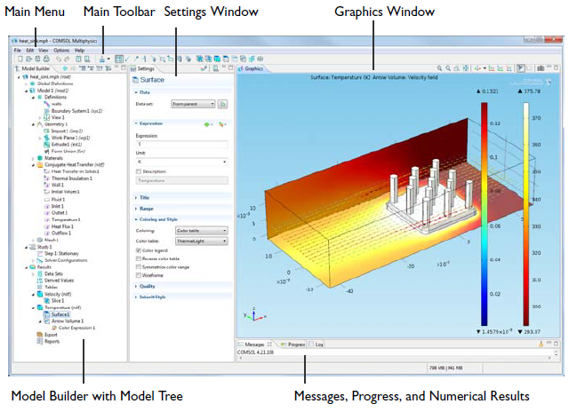
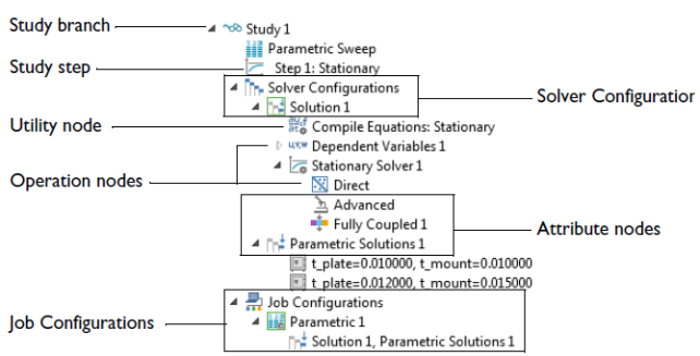
- The iteration number (Iter)
- A relative error estimate, which is one of the following:
- The solution error (SolEst), if Solution is selected from the Termination criterion list for the solver.
- The residual error (ResEst), if Residual is selected from the Termination criterion list for the solver.
- Both the solution error and the residual error (SolEst and ResEst), if Solution or residual or Solution and residual is selected from the Termination criterion list for the solver. The convergence is then based on the minimum of the solution error or the residual error multiplied by the residual factor.
- If the solver log detail is set to Detailed from the Solver log list in the Advanced node’s Settings window, the residual error and the solution error (depending on the selected termination criterion) from each individual field in the model appear in the solver log.
- The damping factor used in each Newton step (Damping).
- Fraction of Newton and Cauchy steps for the Double dogleg solver (Newton, Cauchy).
- The size of the undamped Newton step (Step size) in the error estimate norm.
- The numbers of residuals (#Res), Jacobians (#Jac), and linear-system solutions computed (#Sol) so far.
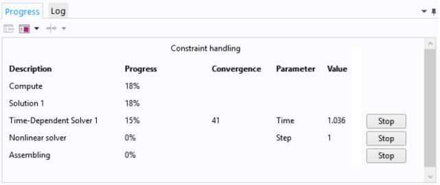
- The Description column shows the solver name.
- The Progress column shows an estimate of the solver progress.
- The Convergence column shows an estimate of the solver’s convergence if available.
- The Parameter and Value columns contain solver-dependent information: the adaptive solver shows the adaptive mesh generation number, the time-dependent solver shows the time, the parametric solver shows the parameter value and the non-linear solver and iterative linear system solvers show the iteration number.
CANCEL OR STOP A SOLVER PROCESS
You can cancel or stop the solver process if the solving time or likelihood for convergence is not progressing as expected. Use the horizontal or vertical scrollbars if needed. On the status bar you can follow the progress, cancel the solver process by clicking the Cancel button or click the Progress button to open this window. In the same way you can also cancel the meshing and the evaluation during post-processing.You can use the Stop buttons that appear at each solver level to stop the execution. When you click a Stop button, COMSOL returns a current approximation to the solution if possible. For example, when you click it at the adaptive solver level, the underlying linear, non-linear, parametric, eigenvalue or time-dependent solver continues until it is finished, but the adaptive solver stops at its current generation, immediately returning a solution.
Similarly, you can click the Stop button to return the current iteration for the non-linear solver or an iterative solver. Also use the Stop button during time stepping to return all time steps up to the current one. The parametric solver works similarly: to return the solutions for all parameter values up to the current one, click the Stop button.
Contacts and Interfaces
Excerpts from COMSOL Reference Manuals:Pairs are available for assemblies (that is, geometries created by not forming a union of all geometry objects as the final step), where there is a need to connect boundaries between parts. By default, pairs are created automatically when forming an assembly. Contact pair modeling requires the Structural Mechanics Module or MEMS Module. There are two types of pairs - identity and contact.
IDENTITY PAIRS
An identity pair by default makes the fields across two connected boundaries (one from each connecting object in an assembly) continuous. This is equivalent to the continuity that is obtained by default on interior boundaries in a geometry created by forming a union. Some physics provide special boundary conditions for identity pairs to model slit conditions such as resistive layers. You can specify boundary conditions for these pairs from the Pairs submenu at the bottom of the boundary condition part of the context menu for the physics feature node.In case you want to merge the pair created by slit operation, use Fuse Boundary Zone operation. It merges nodes, faces and works only on face zones. Note that Merge Zones does not cause any topological changes in the mesh - only new groupings of mesh are created (which is mostly irreversible). It is analogous to operation "Surface Grouping" in CFD-Post. The purpose is to reduce the number for zones for boundary condition settings and ease of selection of zones during post-processing operation.
CONTACT PAIRS
A contact pair defines boundaries where the parts can come into contact but cannot penetrate each other under deformation for modeling of structural contact and multiphysics contact.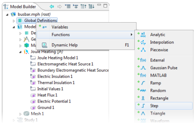
Workflow for AcuSolve
AcuConsole is the pre-post processor for solver AcuSolve which is based on the Galerkin/LeastSquares (GLS) finite element method. AcuFieldView is an OEM version of Intelligent Light’s FieldView CFD post-processor.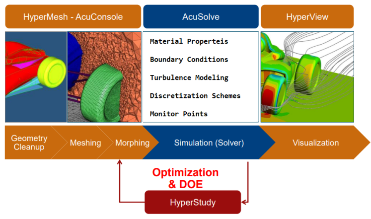
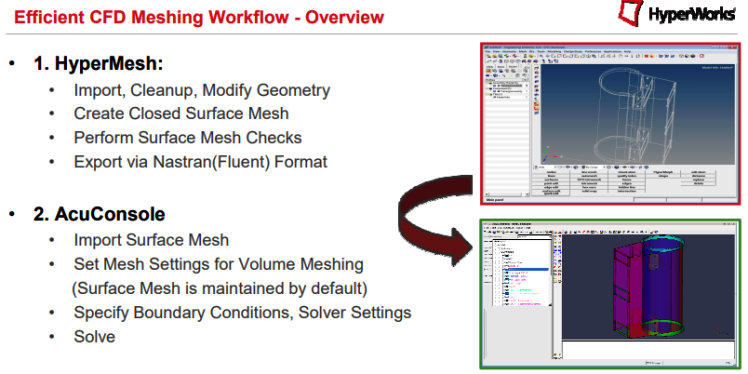
Dimensionless Numbers
- CFL NUMBER: CFL, it is ratio of characteristic flow velocity to the speed with which time-marching solution advances over a mesh.
- Knudsen number: Kn, defined as the ratio of the mean-free path to the characteristic length scale.
- Mach number: M, defined as the ratio of the characteristic velocity to the sound speed
- Reynolds number: Re, defined as the ratio of the product of the characteristic velocity × characteristic length to the kinematic viscosity. This is one of the widely used number required to distinguish laminar and turbulent flow regimes.
- Strouhal number: Sh, defined as the ratio of the mean-free time to the characteristic time scale. This number is used to express vortex-shedding frequency of wake regions behind bluff-bodies.
Stop Remote Runs
The method to stop or abort a run in batch mode is called check-pointing. A blank text file of specific name is created in running directory which is checked by solver at every iterations - to save at the end of the current step (iteration in a steady case, time-step in a transient case). For example, following method can be used to stop a STAR-CCM+ run.

This action creates a new simulation (.sim) file saved at the end of current iteration, with a (@) and iteration number appended to the filename. STAR runs in progress on a remote cluster can be monitored on user's Desktop using File > Connect to Server and then specifying the server path. The server path itself needs to be extracted from the live log file and look for the line which reads like Server::start -host xyz:13579 where xyz is server hostname and 13579 is the port number.
Multiple Runs in a Sequence: STAR-CCM+ and CFX
There are two type of requirements: (a)single set-up files with few changes in set-up such as boundary conditions, material properties... also known as different variants of one exploration project (b)multiple set-up files not related to each other. In FLUENT, the runs can be put in queue using journal files where next line is not executed until the operations as per current line is finished.
Design Manager available in STAR-CCM+ since version 2017 allows to do automated design studies - multiple runs in sequence. This is a two step process: 1)Prepare the Design Manager project on the local machine by creating a new study under "Design Studies" tab in model tree and specifying required parameters, objectives or constraints. 2)Edit settings for parallel computing under Design Studies > Design Study > Settings > Run Settings.
In CFX, multiple runs with parametric study (say changing velocities at inlet) can be set in a single CFX file using "Simulation Control" tab.


HypersoniC Flows
Reference: "Simulation of Hypersonic Flow Fields Using STAR-CCM+" by Peter G. Cross and Michael R. West, Aeromechanics and Thermal Analysis Branch, Weapons Airframe Division. Excerpts: "Hypersonic flight (i.e., flight in excess of Mach 5) produces high temperatures that activate certain physical processes, including temperature-dependent properties, thermodynamic nonequilibrium, dissociation, and ionization, normally dormant for slower flight regimes. When simulating hypersonic flow, it is very important to model these additional physical processes, which require the inclusion of specialized models into the flow solver.""The large kinetic energy associated with hypersonic flight leads to very large temperatures behind shock waves and in the boundary layers adjacent to vehicle walls. These high temperatures lead to the activation of physical processes that are unimportant at the lower temperatures associated with lower speed flows. The vibrational energy mode for diatomic molecules (O 2 , N 2 ) becomes excited at temperatures above 800 K (approximately Mach 3), leading to temperature-dependent thermal properties. At even higher temperatures, chemistry takes place (predominantly dissociation reactions), with oxygen beginning to dissociate at 2,500 K (about Mach 6) and dissociation of nitrogen beginning at 4,000 K (near Mach 8). Ionization of air begins at around 9,000 K (approximately Mach 12), leading to the formation of a plasma."
"Since shocks are the main flow feature to be resolved in these hypersonic flows, an initial technique is pursued that refines the mesh based upon the pressure gradients in the flow. In this approach, an initial solution is obtained using a fairly coarse and uniform initial mesh. This mesh is then refined, the solution from the old mesh is interpolated onto the new mesh as an initial condition, and the solution is run to convergence on the new mesh. This refinement process can be repeated several times, until an acceptable level of mesh refinement is obtained."
Dashboard for Utilization of Clusters
The job schedulers typically provides limited options for monitoring various aspects of the running jobs and hence a good dashboard is pre-requisite to ensure better utilization of all resources: hardware, software and manpower. This gives users better insights to plan the runs. The table can be updated every 30 minutes and no real-time update is required. From slurm job scheduler: "Slurm-web provides a web interface on top of Slurm with intuitive graphical views, clear insights and advanced visualizations to track your jobs and monitor status of HPC supercomputers in your organization." Slurm-web is an open source web dashboard for Slurm based HPC clusters. Prometheus monitoring framework and the Grafana visualization toolkit are other job monitoring platforms.
| Operational Parameter | Unit | Value | Current in Use | Demand in Queue* | Cores being used |
| Total number of cores | [no] | 256 | 128 | 64 | - |
| Total hard disk space | [GB] | 1000 | 524 | - | - |
| Total solver licenses: ABAQUS | [no] | 5 | 3 | 1 | 32 |
| Total solver licenses: ANSYS HPC Packs | [no] | 8 | 4 | 2 | 96 |
| Total solver licenses: STAR-CCM+ Power | [no] | 5 | 2 | 1 | 64 |
| Total solver licenses: LS-Dyna | [no] | 3 | 1 | 0 | 16 |
Status of ongoing runs: this may require reading the log-files of the ongoing simulations in-progress.
| License Type | Cores used | User Name | User ID | Job-ID | Total Run Time [hours] | Expected Finish Duration [hours] |
| STAR-Power | 32 | A | 101 | C1035 | 4.0 | 2.5 |
| ANSYS HPC-Pack | 64 | B | 103 | C1036 | 3.2 | 1.5 |
| STAR-Power | 96 | C | 105 | C1037 | 5.2 | 3.5 |
| ABAQUS | 16 | A | 101 | F2356 | 2.5 | 6.0 |
| LS-DYNA | 32 | D | 108 | F2367 | 8.1 | 9.0 |
| ANSYS HPC-Pack | 32 | B | 103 | F2368 | 2.5 | 8.0 |
The content on CFDyna.com is being constantly refined and improvised with on-the-job experience, testing, and training. Examples might be simplified to improve insight into the physics and basic understanding. Linked pages, articles, references, and examples are constantly reviewed to reduce errors, but we cannot warrant full correctness of all content.
Template by OS Templates