- CFD, Fluid Flow, FEA, Heat/Mass Transfer
Post-processing
Post-processing of CFD Results
Extracting Engineering Information from CFD Results
Post-processing activity includes generation of detailed report with the help of quantitative data, qualitative data, contour plots, vector plots, streamlines, area-average values, mass-average values, pressure coefficient, lift coefficient, centre of pressure.
Table of Contents:
Checklist for Simulation Result | Paragraph, Units, Fonts in a Report | Post-processing for DPM | Data Exchange between Solvers {+} Centre of Pressure | Observations and Design Recommendations | Radiation View Factors | Display Annotations in Graphics Window | Post-processing for Turbo-machines | Post-Processing in CFD-Post | Post-processing for Transient Runs | Mass-weighted or Area-weighted? | Function Calculator in CFD-Post | Custom Volume in CFD-Post | Booleans in CEL || Overall Steps of CFD Simulations |=| Vorticity Plot [] Post-processing on Irregular Surfaces
Orifice Size Estimation [-] Heat Conduction through Wires |+| Estimate Flux Values {*} Streamlines
One of the commonly used term in post-processing and visualization technique is 'rendering'. This refers to the process of converting underlying mathematical representation of solid geometry into visual forms.
The screen is represented by a 2D array of locations called pixels. One of 2N intensities or colors are associated with each pixel, where N is the number of bits per pixel. Greyscale typically has one byte per pixel, for 28 = 256 intensities. Color often requires 1 byte per channel, with 3 color channels per pixel: red, green, and blue. An "image map" or 'bitmap' or "frame buffer" is a array or variable to store color data. Z-buffer is the element of the computer hardware/software that is expected to manage the depth of the image (in the z-direction - into the plane of the screen).The important of visual data is summarized in image below. Look at the comparative statistics of information retained by people: 80% in case of visual information, 20% of reading and just 10% of information reaching through ears.

Excerpts from ParaView tutorial manual: "the process of visualization is taking raw data and converting it to a form that is viewable and understandable to humans. This allows us to get a better cognitive understanding of our data. Scientific visualization is specifically concerned with the type of data that has a well defined representation in 2D or 3D space. Data that comes from simulation meshes and scanner data is well suited for this type of analysis. There are 3 basic steps to visualizing your data: reading, filtering and rendering. First, your data must be read into ParaView. Next, you may apply any number of filters that process the data to generate, extract or derive features from the data. Finally, a viewable image is rendered from the data."
Before you proceed to generate a report
Check mass balance as sum of mass flow rates at inlet(s) and outlet(s), energy balance at all walls (excluding inlets and outlets), reverse flow at outlets, Y+ at all walls (minimum, maxium and area-averaged), minimum and maximum values of velocity, pressure and temperature in the domain... One may try to develop a script or journal to make these checks and report a summary. Check if the standard units in which quantitative results shall be generated is easy to record or not. For example, for low flow rates cases, a value such as 0.000135 [m3/s] is difficult to read and type for further processing. It is better to use a unit which shall give the number in the range 0.1 to 100 scale. Here, the unit of flow rate can be changed to LPM or cc/s.
Change post-processing units in ANSYS FLUENT: ANSYS FLUENT uses SI system for all calculation internally. However, for post-processing and user inputs, it provides multiple options. Some variable and available units are:
- Length: m, cm, mm, in, ft
- Area and Volume Flow Rates: same combindation as in length such m^2, cm^2, ft^3/s
- Velocity:m/s, cm/s, km/h, ft/s, ft/min, mph
- Dynamic Viscosity: kg/(m s) ≡ Pa.s, poise, lb/(ft s), slug/(ft-s)
- Density: kg/m^3, lbm/ft^3, slug/ft^3, g/cm^3
- Pressure: Pa, atm, psi, torr, lb/ft^2, inWg, dyne/cm^2
In STAR-CCM+ units has to be set using GUI: step-1 is to select units under Tools > Units -> tick Preferred in 'Properties' window. And then step-2 is to right click on Units tab and select "Save as Defaults". A new unit can be created using field 'Conversion' and 'Offset' in Properties window.
Common Issues in Post-Processing
The maximum value of a domain (eg: maxVal(Temperature)@wallX) gives a cell-centred value (Fluent is coded with this method). The maximum value from a (probe) point corresponds to the temperature value of the nearest node (CFX and CFD-Post operate on this principle). The cell centred value must be used to obtain a more accurate maximum or minimum value as this bases the value on the centroid of the cell.
STAR: The output shows maximum temperature limited to 5000 in 3468 no. of cells... These messages very often indicate a problem with mesh or unreasonably high heat flux. Check the quality of mesh before running: Right click on your Region -> Remove Invalid Cells -> Preview -> The boxes should indicate 0 problem cells found for a good mesh. Additionally, visualize where this (unrealistic) minimum or maximum temperature is taking place by making a threshold: Representations -> Expand Volume Mesh -> Right click on Cell Sets -> Threshold). Create a lower threshold for unreasonable low temperature and higher threshold for unreasonably high temperatures. Note that temperature thresholds are ALWAYS in [K] no matter which solution units are set. In FLUENT one can try turning secondary gradient OFF.
Checklist for Simulation Result
| S. No. | Checkpoint | Record |
| 01 | Has the overall mass imbalance of ≤ 0.01% achieved? | |
| 02 | Have the velocity and pressure profiles at inlets and outlets been checked for uniformity? | |
| 03 | Has the pressure drop reported for porous domains been checked with expected value as per P-Q curve? | |
| 04 | Has the contour plot been set as banded instead of continuously coloured? | |
| 05 | Has the precision of labels (number of decimal places) set as per the range of data on legend? | |
| 06 | Has the format of number labels on legend set as per magnitude of values: float, decimal or exponential? | |
| 07 | Has the material properties at inlets and outlets checked to be closed to expected and/or specified values? |
These are some basic sanity checks which one should make before starting to prepare detailed report. One should always think how easy the plots are to read, interpret and draw conclusions.
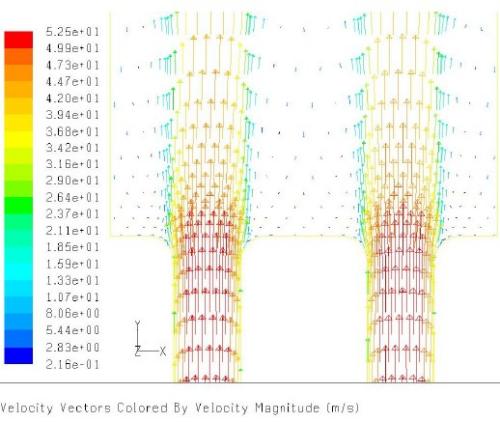
Vector Plot
A vector plot is qualitative representation of spatial magnitude. The only limitation is that it can be drawn plane or a 3D twisted surface. For any vector or contour plot, one of the important consideration is to selection the number of colour bands (also called the legend).- This should be small enough to have a distinct interval and high enough to keep it legible and easy to read and distinguish.
- A value between 8 and 16 normally is a good choice.
- Note the example below has 20 bands (with 21 values) and how cluttered it looks. There are 2 colours very close in intensity and cannot be easily distinguished looking at the plots.
Streamlines
Streamlines are very good representation of velocity field, at least to beginners in CFD. It is closely related to velocity vector and any inconsistency may arise only because of post-processing interpolation on coarse mesh. As theoretically explained, tangent to streamlines gives direction of velocity field at that point.
For more control, define a rake (a line or plane) rather than using an inlet face. This allows to specify exactly how many points are used to start the streamlines.
Contour Plot
Contour plots are "coloured-band" plots of any variable where range of value is represented by a single colour band. This is good presentation of information in both the qualitative and quantitative format.
Iso-surfaces
Iso-surfaces are surface or planes with constant value of a particular variable. CFD-Post has feature to create interactively, same feature is available in FLUENT through Iso-surface option. Hence, to create a plane parallel to X-Y plane, Z value will remain constant. Iso-surfaces are also useful to visualize the effect of one variable on any other variable over the entire domain. Use the marking feature (used to mark cells for adaption) to identify cells having value equal to the solution limit. Use the Iso-Value Adaption dialog box which opens though Adapt/Iso-Value... menu item
Geometrical Variable in CFD-Post
The cell level data available in CFD-Post (available under Variable selector) are: Area, Connectivity Number, Edge Length Ratio, Element Volume Inverse, Element Volume Ratio, Length, Maximum Face Angle, Minimum Face Angle, Volume, X, Y, Z, Normal: Normal X, Normal Y, Normal Z.Access residual values for each cell of the flow domain: Use TUI command /solve/set/expert and set "Save cell residuals for post-processing? [no]" to yes. Then run the simulation for 1 iteration so that the specific data fields are created after which the residuals of all solved equations can be accessed and postprocessed within FLUENT Post. They can also be used for convergence monitors. To store the residuals in the data file, adjust the data file quantities (File > Data File Quantities) and the select variables under "Additional Quantities". Residual histories for each variable are automatically saved in the data file, regardless of whether they are being monitored.
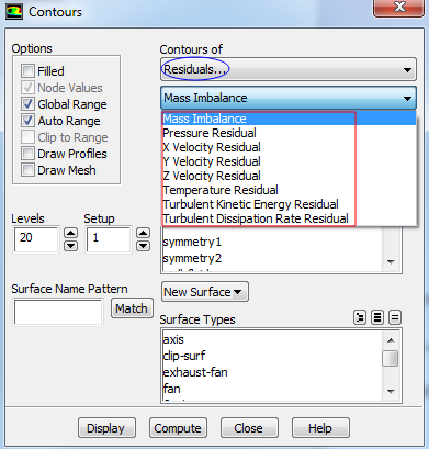
Excerpt from user manual: "If you are having solution convergence difficulties, it is often useful to plot the residual value fields (e.g., using contour plots) to determine where the high residual values are located. When you use one of the density-based solver, the residual values for all solution variables are available in the Residuals... category in the postprocessing dialog boxes. (If you read case and data files into ANSYS FLUENT, you will need to perform at least one iteration before the residual values are available for postprocessing.) For the pressure-based solver, however, only the mass imbalance in each cell is available by default. Note that residual values are not available for the radiative transport equations solved by the discrete ordinates radiation model."
Iso-Volume
As on version 2021R1, there is no iso-volume function in Fluent pre-post. Adaption registers can be used to generate the data equivalent to isovolume operation and then exported into other formats. Cell Registers -> Field Variable and then change the Type to Cells in Range. Some post-processors (such as CFD Post) has capability to generate the volume of domain based on range of specified variables such as temperature or pressure.
Iso-Clips
An Iso Clip takes a copy of any existing location (plane, boundary...) and then clips (trims) it using one or more criteria. E.g. a outlet boundary plot which is then clipped by Velocity ≥ 1 [m/s] and Velocity ≤ 2 [m/s]. Clip operation can be performed using any variable, including geometric variables and user created variables.
Uniformity index on a plane or boundary
ANSYS FLUENT has option to calculate area-weighted average and mass-weighted average uniformity index on a plane, available under "Surface Integral" menu. CFD-Post does not have direct option to calculate uniformity index. However, area-weighted average uniformity index can be calculated using following expressions. Note that area() is function and Area is field variable in CFD-Post.avgVel = ave(Velocity)@PlaneX areaAvgVel = sum(abs(Velocity - avgVel)*Area)@PlaneX uniformity = areaAvgVel / (2 * avgVel * area(PlaneX))
Surface of Revolution
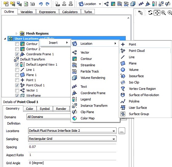
in CFD-Post, predefined options to create Cylinder, Cone, Disc, Sphere and "From Line" are available. The last one is a more general way to use any line (existing Line, Polyline, Streamline, Particle Track) and rotate about an axis.
Other features are: Point Cloud - To Create multiple points which is usually used as seeds to streamlines and vectors, Instance Transform - Usually used to re-create full plots from symmetric/periodic solution data, Clip Plane - Define a plane which when active all viewer objects in front / behind this plane are hidden
Hybrid vs Conservative Value in CFX
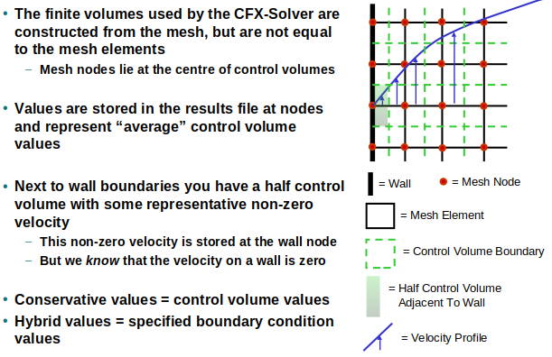
For visualization purposes, ANSYS CFD-Post uses hybrid values by default, because non-zero wall velocities may look incorrect for otherwise stationary walls with no-slip boundary condition. For calculation purposes conservative values are used by default This is physically correct. For example mass flow is calculated correctly — a velocity of zero would produce zero mass flow through the wall adjacent control volume which is clearly wrong.
Display the velocity near a wall
Fluent can display the velocity contour on the wall, with node values disabled which shows the values of the cell centroids adjacent to the wall. In CFD-Post and EnSight, a user-defined surface can be created using "offset from surface" option, with surface-normal as the direction. Specify a small value of normal offset distance based on how close you want to be near the walls, and the velocity will be interpolated to that surface.Display additional information in ANSYS Fluent graphics windows using titles or annotations: In order to create hard copies, it is sometimes useful or even necessary to show flow time or some explanation text that is fixed to a certain position. In recent versions such as ANSYS FLUENT V2022, the title bar is hidden by default. The GUI method is to use the toggle button in the icon toolbars that are connected with the Fluent viewport. Corresponding text command is /display/set/windows/text/visible? yes. The setting is not saved together with the case file. To modify the shown information and/or add different text, use TUI: /display/set/windows/text application? yes and /display/set/titles left-top "text string". To toggle the date shown, use the text command /display/set/windows/text/date? no. The location of date and application text is fixed and cannot be change either though GUI or using TUI. To move this information at a different location in the titles, disable them and use text commands to add fixed text at desired locations. To display flow time in the TUI, type (rpgetvar ‘flow-time) /display/set/titles left-bottom (rpgetvar 'flow-time)
Add Annotations: using TUI or GUI, adding annotation requires a mouse click at desired location. Note that window 1 is the default window that is used to display the residual plot. To use a contour plot window, (cx-use-window-id 2) if residual plot is active. To add annotation: (cx-annotate '() '(0.50 2.50 0.00) "v<" "Annotation text") (cx-changed 'scene-list) where "v<" denotes vertically left-aligned. For right-aligned text, use ">v". The Scheme statement (cx-changed 'scene-list) is required since the Annotate panel is populated with the annotations added by Scheme. Thus, full script looks like:
(cx-use-window-id 1)
(cx-annotate '() '(0.50 2.50 0.00) "v<" (format #f "Time: ~5.3fs" (rpgetvar 'flow-time)))
(cx-changed 'scene-list)
The annotation text can be formatted using:
(cxsetvar 'annotate/font/size "25")
(cxsetvar 'annotate/font/wt "Medium")
(cxsetvar 'annotate/font/slant "Regular")
(cxsetvar 'annotate/color "blue")
(cxsetvar 'annotate/font/name "sans serif")
or
(cxsetvar 'annotate/font/size "50")
(cxsetvar 'annotate/font/wt "Bold")
(cxsetvar 'annotate/font/slant "Italic")
(cxsetvar 'annotate/color "foreground")
(cxsetvar 'annotate/font/name "Courier")
Add CAD Geometry to Contour Plots
When solid walls are not modelled in CFD simulation, they cannot be added to streamlines or vector plots to show isometric views. In case of internal flows, the surrounding geometry adds context to the 2D plots. This requires splitting the original geometry in SpaceClaim at the section where plane was created in CFD-Post. Save the cut section in STL format. Note that one STL file represents one single part even though it may consists of different parts in real life. Save separate STL for separate parts as needed. Import the STL file(s) using File -> Import -> Import Surface or Line Data... option in CFD-Post and colour the geometry with required texture such as Metal, Gold or White Metal.Mass-weighted or Area-weighted?
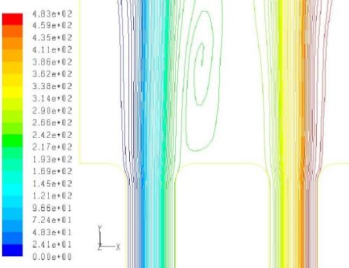
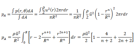
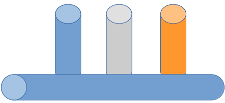
The features explained above are more qualitative in nature and may not be used directly in design calculations which usually require a discrete value. This can be obtained by "area-weighted average" or "mass-weighted average" feature available in the post-processing tools. But, the choice of area-weighting or mass-weighting should be based on the gradients of the chosen field variable. For example, to estimate average temperature at a given section for internal flow, mass-weighted option is the correct method as explained below.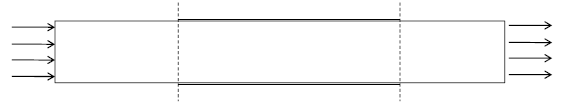
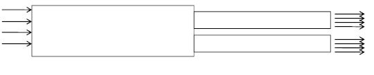
In the pipe flow example above, for calculation of temperature at the planes shown by dashed lines, area-weighted option may not give the correct result as it is a function of mesh size near wall. In the example below, area-weighted average velocity at inlet and the two outlets will not be in the ratio of flow areas even though flow is assumed incompressible. This is because of the error in integration or summation due to sharp gradient of velocity in the boundary layer and mesh may not be fine enough to capture it. Also note that the narrower sections have 4 boundary layers as compared to 2 boundary layers in inlet section.
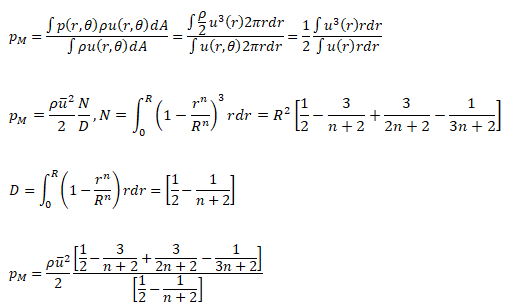
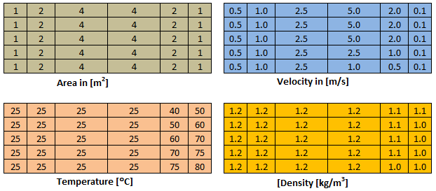
For this sample grid, the average velocity is 1.550 [m/s], the area-weighted average velocity = 2.171 [m/s], mass-weighted average velocity = 3.251 [m/s], average temperature = 37.7 [°C], area-averaged temperature = 32.9 [°c] and mass-weighted average temperature = 27.8 [°C]
Vorticity: It is a measure of the "local rotation" of a fluid parcel defined as the curl of the velocity. In other words, the curl of a vector field measures the rotation or vorticity of the field at a point. Vorticity is a local property defined at every point in space. Note that curl(∇f) ≡ ∇ × (∇f) = 0. Custom Field Function (CFF) for q-criterion in 2D: dX-Velocity-dx * dY-Velocity-dy - dX-Velocity-dy * dY-Velocity-dx. This is definition of vorticity (curl of velocity), Ω = ∇ × V. The variable dX-Velocity-dx ≡ du/dx and others are defined at Variable names in FLUENT.
Divergence of the curl of any vector field is zero (curl of gradient is also zero), thus curl is a fundamental property in vector calculation. Divergence (∇.x) calculates expansion or contraction of field x. The definition of curl cannot be converted in any mathematical expression using divergence.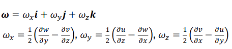
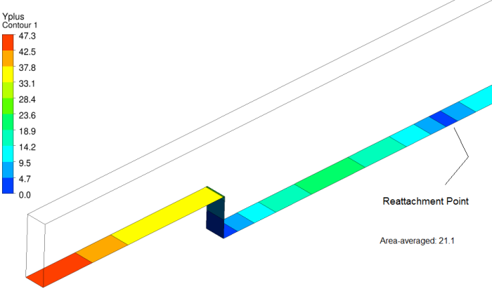
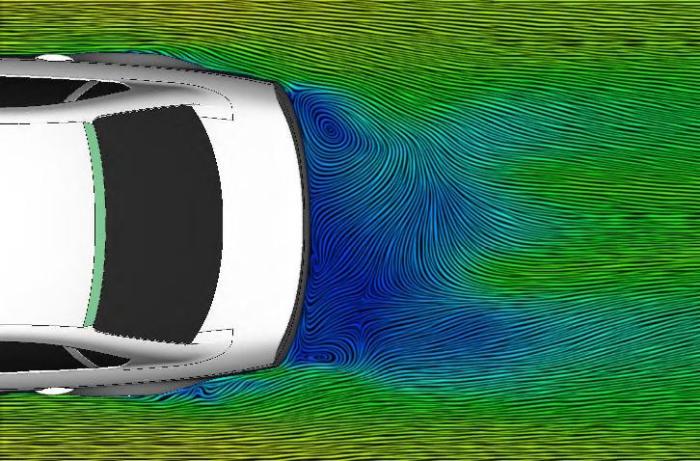
There are few post-processing operations which require not only a good insight into the flow physics but experience as well. For example, the estimation of separation length (the reattachment point) needs careful evaluation. There are many methods, one recommended method can be generation of y+ plot. By virtue of re-attachment, the velocity necessarily has to go close to zero and hence y+ or shear stress will follow the same variation. The following image represents y+ plot for flow over back-facing step.
- One picture or sketch (preferably an isometric or sectional view) representing the extent, origin and axes of computation domain, boundaries and moving walls (if any).
- Sectional view of mesh in area of interest highlighting the boundary layer, growth and orthogonality.
- Mesh quality matrix, worst values of mesh Equi-angle skewness and aspect ratios.
- The description of material properties and its thermodynamic behaviour.
- Tabulated summary of boundary conditions and turbulence parameters.
- Tabulated summary of solver setting: discretization scheme, wall function, relaxation factors
- Contour plots
- Limit the number of colour bands to 10
- Set the decimal notation to FLOAT, INTEGER or SCIENTIFIC (exponential) based on magnitude. E.g. for values ≤ 1000, it is better to use decimal notation instead of exponential format
- Chose the unit easy to read and interpret: e.g. [K] for temperature is difficult to quickly visualize in mind. For most of us, 37 [°C] which is out body temperature or 25 [°C] which is standard ambient temperature serves as reference
- Similarly, a value of 0.075 [m] takes more time to interpret than 75 [mm]. It is quicker to deal with integers than fractions
Postprocessing Simulation Results on Irregular Surfaces: Import surfaces as STL geometry and then imprint them in existing volume mesh within FLUENT Pre-Post. This feature is available in almost all modern post-processors including CFD-Post and ParaView.
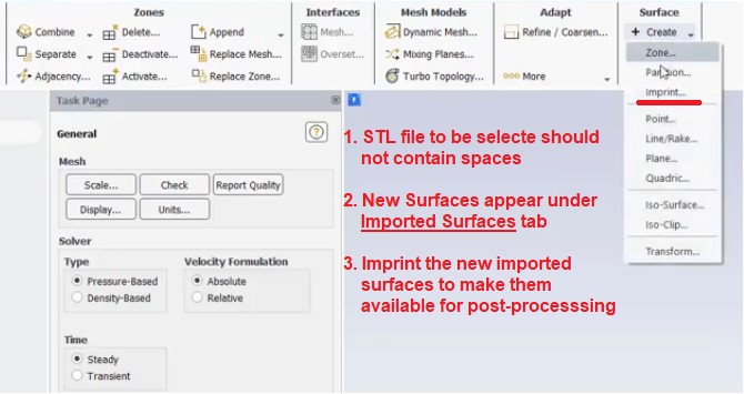
Note that an STL file is a surface file and cannot represent a volumetric region even if the surface is a closed one. This means that if you cut through it say to generate Iso Clip, you shall get the appearance of edges rather than a solid object. Steps to generate STL surfaces are: Slice or create post-processing surfaces using edges/boundaries of original geometry in SpaceClaim -> Save as .STL using Options and switch STL output to ASCII format -> Import the surface in FLUENT Pre-Post as explained earlier. Alternatively, the surface geometry can be imported into FLUENT mesher and meshed with triangles. The STL mesh can be saved using TUI: /file/export stl post_planes.stl which can be read using TUI: mesh/surface-mesh/read "post_planes.stl" mm. /surface/imprint-surface post_plane post_plane_imprint fluid_domain. Note that the mesh should be scaled in FLUENT Mesher to [m] before exporting to STL format.
Surface Groups and Clipped Surfaces
Some program (e.g. CFD-Post) have option to combine boundary surfaces to a named surface group for ease of post-processing. In FLUENT Pre-Post you cannot create a surface group but you can create a single surface for all the walls defining a fluid or solid zone. Then after you can clip the newly created surface based on X-, Y- or Z-coordinates to use say a symmetrical half of the domain.
Cell Set in STAR-CCM+
Cell sets are used to identify collections of cells for visualizing the model, such as during post-processing or mesh checking. A cell set is similar to a derived part though more versatile and can be derived from more than one condition. Cell Sets node is available under Representations > Volume Mesh > Finite Volume Regions node in the simulation tree. A field function is also created for each cell set by default, which appears under the Automation > Field Functions manager node. The field function has the same name as the cell set by default.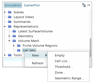
Conventions for Paragraph, Fonts and Symbols
- Chose font size ≥ 11 px, font-type should be easy to read. Calibri, Arial are few good fonts.
- Use line spacing of 1.50 or higher. For bullet points, it can be reduced to 1.25
- If paragraphs are not indented, quadruple-space the paragraphs i.e. add extra space before the pargraphs
- Keep margin of 20 ~ 25 [mm] on each side
- Add page number centred under footer
- Maintain uniformity of font sizes such as for Paragraphs, Headers, Captions...
- Use unique symbols for variables
- Do not use mix of small letters and capital letters for same variables such as u or U, p or P
- Use over-dot for mass flow rates such as ṁ
- List standard (Roman) alphabets and Greek alphabets separately
- Arrange the variable names in alphabetical order
- Keep separate lists for subscripts and superscripts
- Add page number in references, typically any documents (books, journals, theses, research papers...) having number of pages ≥ 5
- Do not use superscript of 'o' or '0' as degree symbol. All of the MS-Office programs Excel, Word and PowerPoint provide degree symbol (°).
- Do not use underline for words containing g, j, p, q, y
- Write all units within square brackets [...]
- No space should be left in front of (before) a punctuation mark
- It is better to write inline reference with page number (e.g. Sukhatme, 1998, p. 21)
- For all title of in-text citations, the first letter of every word except articles (a, an, the), prepositions (such as in, on, under...), and conjunctions (such as and, because, but, however ...) should be capitalized, unless they occur at the beginning of the title or subtitle
- In-text citations must provide the name of the author or authors and the year the source was published
- The references page should be double-spaced and lists entries in alphabetical order by the author’s last name
Spelling Errors:
- Note that there is no space before any of the punctuations such as . (full stop) , (comma) : (colon) ; (semi-colon) closing ' (apostophe) and closing " (double quote)
- There are some words which spell check cannot identify as error. There are words generated due to nearby key on the kewords: e.g. [any:nay], [out:our], [neat:near], [near:hear], [below:bellow], [field:filed], [from:form], [for:fro], [its:it's], [though:through], [it is:it it], constrast : contract, varies : varied
- Check all the occurrences of 'it' and ensure 'it' and 'is' are used appropriately. Note that its and it's are not same
- Do not use &
- Full stop is used only at the end of last entry of a bulletted list.
In ANSYS FLUENT pre-post (V19 or earlier), walls and section planes are diplayed along with partition boundaries. To remove the partition boundaries - try (cxg-stitch-shells). This SCHEME command needs to be used after every new plot operation. Alternatiely, you can try TUI: "define beta yes" followed by "display set duplicate yes".
- Use same lower and upper limits of legends for contour as well as vector plots
- Use decimal notation if variables are > 0.01. Even though scientific notations can be used, it is easier for human mind to read numbers as compared to exponential notations.
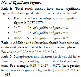
- Use number of significant digits judiciously. For example, for most of the industrial applications, it is not important to specify velocity to the 1/10 of mm/s. The number of significant digit is also dependent on the units chosen. For example, 3 decimal places for [Pa] such as 1045.368 [Pa] is irrelevant where as it is a need if unit chosen is [bar] or [kPa] such as 1.034 [kPa]. Followings are more information about "number of significant figures or digits".
One of the issues observed in contour plots is not making intuitive selection of lower and upper bounds. It is easier to read a numbers which are rounded to a multiple of 5 or 10. Following steps demonstrate how to write a script to convert a number into nearest multiple of 0.01 where any number between 8001 to 8099 shall be rounded to 8000.
- Take the log (base 10) of the number. For 8235, it would result in n1 = 3.916
- Use the math operator equivalent to FLOOR and find the nearest higher integer: n2 = FLOOR(n1, 1) + 1 = 4
- Divide the original number with exponent of 10, n3 = 8235/104 = 0.8235
- Use another FLOOR operation with desired significan, 0.01 in this case. n4 = FLOOR (0.8235, 0.01) = 0.82
- Multiply the previous number with exponent of 10, n5 = n4 x 10n2 = 8200.
CONTOUR: Contour_Total_Pressure
  Max = 1.5E4
  Min = 0.5E3
  Number of Contour = 11
END
Due to limitations of floor operator in Python, the above-mentioned steps need to be tweaked as bit as described below.
import math, sys
def removeSignificantDigits(number, num_sign_digits):
  '''
  number: the value to be converted to nearest order of magnitude
  num_sign_digits: number of significant digits to be removed
  '''
  n1 = math.log10(number)
  n2 = math.floor(n1)
  if (n2 < num_sign_digits):
    print("The specified number of significant digits cannot be removed!")
    sys.exit()
  n3 = math.floor(number / 10**num_sign_digits)
  n4 = n3 * 10**num_sign_digits
  return n4
print(removeSignificantDigits(23456, 3)) # 23000
The method needs to be revised while using PERL as it does not have a floor and log10 operator. Also, PERL does not required to be specified the input arguments in advance. $_ list needs to be used.
sub removeSignificantDigits {
  $number = $_[0];
  $num_sign_digits = $_[1];
  $n1 = log($number) / log(10.0);
  $n2 = int($n1);
  if ($n2 < $num_sign_digits) {
    die("Input has less number of significant digits than to be removed \n");
  }
  $n3 = int($number / 10**$num_sign_digits);
  $n4 = $n3 * 10**$num_sign_digits;
  return $n4;
}
print removeSignificantDigits(23456, 2), "\n"; # 23000
The code in Java is:
import java.io.*;
import java.lang.*;
public class removeLeadingDigits {

  public static void main(String[] args) {
   System.out.println(removeSignificantDigits(23456, 3));
  }
  static double removeSignificantDigits(double number, int num_sign_digits) {
    double n1 = Math.log10(number);
    double n2 = Math.floor(n1);
    if (n2 < num_sign_digits) {
      System.out.println("Specified number of significant digits too high!");
      System.exit(1);
    }
    n2 = Math.floor(number / Math.pow(10, num_sign_digits));
    return (n2 * Math.pow(10, num_sign_digits));
  }
}
If you are extracting quantitative information using scripts, following code can be used to ensure consistent decimal and scientific formats for the numbers based on their absolute values.
def formatNumbersConsistently(number):
  abs_n = abs(number)
  if (abs_n < 1e-4):
    num_format = '{:0.2e}'.format(number)
  elif (abs_n >= 1e-4 and abs_n < 1):
    num_format = '{:0.4f}'.format(number)
  elif (abs_n >= 1.0 and abs_n < 10):
    num_format = '{:0.3f}'.format(number)
  elif (abs_n >= 10 and abs_n < 100):
    num_format = '{:0.2f}'.format(number)
  elif (abs_n >= 100 and abs_n < 1000):
    num_format = '{:0.1f}'.format(number)
  elif (abs_n >= 1000):
    num_format = '{:0.2e}'.format(number)

  return num_format
PERL for CFD-Post
sub formatNumbersConsistently {
  $abs_n = abs($_[0]);
  if ($abs_n < 1e-4) {
    $num_format = sprintf("%.2e", $_[0])
  } elsif ($abs_n >= 1e-4 and $abs_n < 1) {
    $num_format = sprintf("%.4f", $_[0])
  } elsif ($abs_n >= 1.0 and $abs_n < 10) {
    $num_format = sprintf("%.3f", $_[0])
  } elsif ($abs_n >= 10 and $abs_n < 100) {
    $num_format = sprintf("%.2f", $_[0])
  } elsif ($abs_n >= 100 and $abs_n < 1000) {
    $num_format = sprintf("%.1f", $_[0])
  } elsif ($abs_n >= 1000) {
    $num_format = sprintf("%.2e", $_[0])
  }
  return $num_format;
}
For Java in STAR-CCM+ cases, replace the if..elseif loop and use String.format("%.2f", number).
Recommendations for Rotating Reference frame
- Clearly specify the rotating and stationary domain, direction of rotation, location of the interfaces.
- Show the overlapping view of meshes at the interfaces, if not 1:1.
- Mention the location of the place used to estimate pressure heads developed by the machine. It is further recommended to use 3 or more close locations on the upstream as well as downstream sides to estimate the grand average values of the pressure.
- The physics governing performance of turbo-machines uses many non-dimensional coefficients. Include the plots of important performance parameters such as pressure coefficients on the blades
- On all the plots dealing with flow passage and blades, explicitly mention the suction and pressure sides.
Flux values are important to check the conservation of mass, momentum and energy. Note that in case there are reverse flows at the outlet, the area-weighted average values of temperature and pressure may significantly deviate from expected value. In other words, the gain in internal energy of fluid as calculated from [mass flow rate] x [specific heat capacity] x [TEX - TIN] may not be equal to the heat gained by the air through the walls and the heat sources. However, this is more of a data interpolation error on finite cells at the outlet and has less implication on the global energy balance. In case of flows with heat transfer, it is important to set the temperature of fluid entering into the computational domain at the outlets (the reverse flows) close to the expected values to reduce the deviation with respect to thermodynamics energy balance described above.
The discrepancies increases with reduction in mass flow rates such as buoyancy-driven flows. Hence, it is important to move the outlet plane to a location where such reverse flows are not expected.
- The mass flow rate through a boundary is computed by summing the [dot product of the density × the velocity vector] and the area projections over the faces of the zone.
- The total moment vector about a specified center of action is computed by summing the [cross products of the pressure and viscous force vectors] for each face with the moment vector.
- Export heat flux data on wall zones (including radiation) to a(including radiation) to a text file: file/export/custom-heat-flux
- To display the amount of heat removed, outlet temperature, and inlet temperature of the entire heat exchanger during post processing: define/models/heat-exchanger/macro-model/heat-exchanger-report zone_porous_hx. To post-processing each macro result of the heat exchanger: define/models/heat-exchanger/macro-model/heat-exchanger-macro-report zone_porous_hx.
Probe Function: Some programs such as ANSYS FLUENT use mouse button click to probe values at an arbitrary point. STAR-CCM+ has a probe function separately defined. In ANSYS FLUENT, when you probe (typically right mouse button) in a contour plot, the output printed in console is the band of the contour plot where the probed location falls. It does not print the coordinates of the location and estimated value at the probe position. In order to print the location and value at the probe position, plot the contour along with the mesh (you can use Scene to combine a mesh and contour plot).
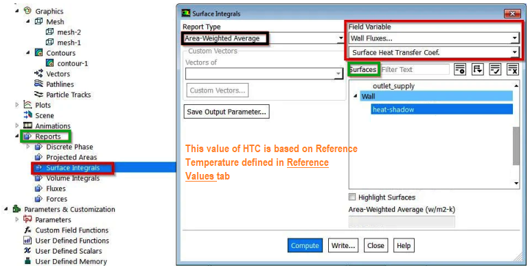
To find the node nearest to a given point, CFD-Post has variable NearestNodeNumber. !nodeAtPoint = getValue('Pt_x', 'NearestNodeNumber'); If point is inside the domain, it will return a positive number else -1. If the point is outside the domain, it will still find the nearest point but only within a tolerance of approximately (0.01*Mesh Extents).Plot HTC (Heat Transfer Coefficient) in ANSYS FLUENT
Custom Volume: sometimes it is needed to create a custom volume such as cylindrical or conical section and generate volume average for the nodes falling inside or outside it. The equation X2 + Y2 = R2 defines an infinite cylinder along Z-axis. How does one define a finite cylinder between points [0, 0, Z1] and [0, 0, Z2]?
- Let A and B are the two ends of the cylinder with coordinates [x1, y1, z1] and [x2, y2, z2] denoted by vectors rA and rB respectively.
- Unit vector along the axis of cylinder is defined by e = rA - rB
- Let P be an arbitrary point along the cylindre axis is given by t.A + (1−t).B where t varies between 0 and 1
- The squared distance between a point on the line with parameter t and a point r0 = (x0, y0, z0) is R2 = [(x1 - x0) + (x2 - x1).t]^2 + [(y1 - y0) + (y2 - y1).t]^2 + [(z1 - z0) + (z2 - z1).t]^2
- The minimum distance between point r0 and axis of the cylinder is: R^2 = [ (x1 - x0)^2 + (y1 - y0)^2 + (z1 - z0)^2 ] + 2.t. [(x2 - x1)(x1 - x0) + (y2 - y1)(y1 - y0) + (z2 - z1)(z1 - z0)] + t^2. [(x2 - x1)^2 + (y2 - y1)^2 + (z2 - z1)^2]
- The points falling inside a finite cylindrical volume of radius R and axis points x1 and x2 CANNOT be specified by inequality:
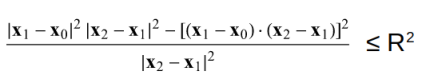
- Above inequality only tells that point may lie within radius of the cylinder and does not check if the point lies between the points x1 and x2 on its axis.
- Boolean operator can be used to truncate a cylinder. For example, a cylinder with left face at (0, 0, z1) and right face at (0, 0, z2) having radius can be specified as (x^2 + y^2 ≤ r^2 AND (z ≥z1 AND z ≤ z2)
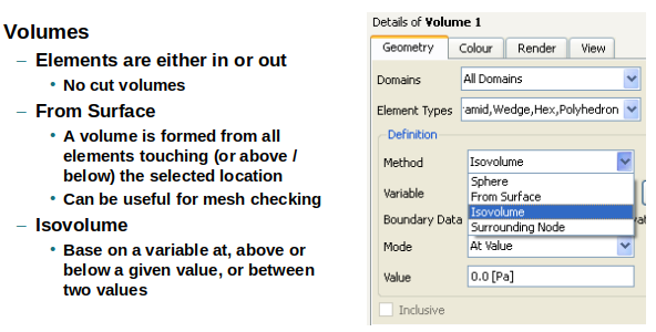
The picture above describes 3 methods to create volume in CFD-Post. The inside() function returns 1 when inside the specified location and 0 when outside - this is useful to limit the scope of a function to a subdomain or boundary. The step() function return 1 when the argument is positive and 0 when the argument is negative. This is useful as an on-off switch and alternatively if() function can also be used as a switch. sqrt(X^2 + Z^2) defines distance from the Y-axis and sqrt(X^2 + Y^2 + Z^2) defines a sphere. sqrt(X^2 + Y^2 + (Z - 0.5[m])^2) moves the sphere by a distance of 0.5 [m] in the positive Z direction. Nested conditional statement can be used to create more 3D shapes: if (0.005[m] <= x && x <= 0.025[m], 2.50, 7.50).
To define a cube: create expression based on if conditions: if(X≤xmax && X≥xmin && Y≤ymax && Y≥ymin && Z≤zmax && Z≥zmin, 1, 0). Create 'Isovolume' and select variable defined with this expression. Set 'Value' = 1 as the if condition shall result in 1 if location falls inside the cube.
Quadric Surfaces: If surface is not sphere, cylinder, plane, circle or line, it is called quadric defined by equation a.x2 + b.y2 + c.z2 + m.xy + n.yz + p.zx + u.x + v.y + w.z + k = 0
Create point cloud
Booleans in CEL: Let's write an expression as dx = (x ≥ 0.05 [m] && x ≤ 0.25 [m]). The value of dx for 3 different values of x are as follows:
- x = 0.0, dx = 0
- x = 0.15, dx = 1
- x = 0.50, dx = 0
Note that this expression can be used to define a finite cylinder of radius 0.1 [m] on x-axis between x = 0.05 [m] and x = 0.25 [m]. fincyl = (y*y + z*z ≤ 0.1*0.1 && x ≥ 0.05 [m] && x ≤ 0.25 [m]). CFD-Post offers 4 modes to define clip range: At Value, Below Value, Above Value and Between Values.
In STAR, stepFun = ($$Centroid[2] <= 50) ? 0 : 1 - this creates a step function at the global z-coordinate of centroids of cell ≤ 50. Multiple if conditions - Split a region (Split Regions by Function dialogue) into 3 parts: ($$)Position[1] <= 2.5) ? 1 : (($$Position[1] >= 0.5) ? 2 : 0). In this case, after the split: The cells where 0.5 < y < 2.5 belong to Region 1, as the field function does not affect them. The cells where y ≤ 0.5 belong to Region 1 2, as it is the created region with the least cells. The cells where y ≥ 2.5 belong to Region 1 3, as it is the created region with the most cells.
Custom Surface Integrals: As described at forum.ansys.com/forums/topic/surface-integral-of-a-plane: to calculate induced drag D = Σ[(v2 + w2) x area of cell], run the command /solve/set/expert no no yes no which activates the option of "Keep temporary solver memory from being freed". Create the variable for equation drag_i = [(v2 + w2) x area of cell]. To select the cell surface area, "Cell Surface Area" is available under 'Mesh'. To compute drag D, use Results > Reports > Surface Integrals - pick variable drag_i, and select the required surface.
Data Exchange
There is no direct option in any of the commercial software to read results from other commercial software in their native formats. However, most of the software provide options to export data into some common post-processor such as FieldView or Tecplot. The option to export and import data from CGNS format also exists.
Export option in FLUENT
The option File > FSI Mapping provides a method to transfer CFD data to FEA for 1-way FSI (Fluid-Structure Interaction) simulations.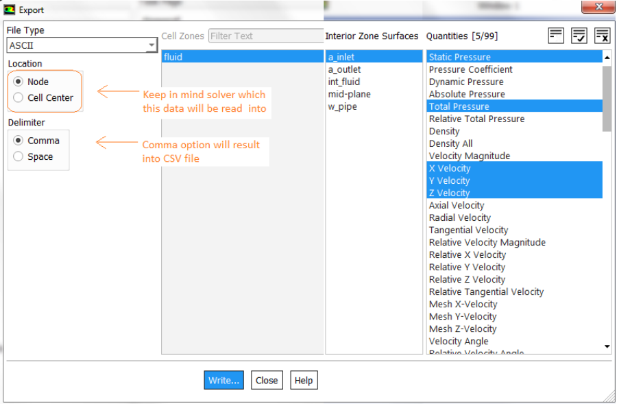
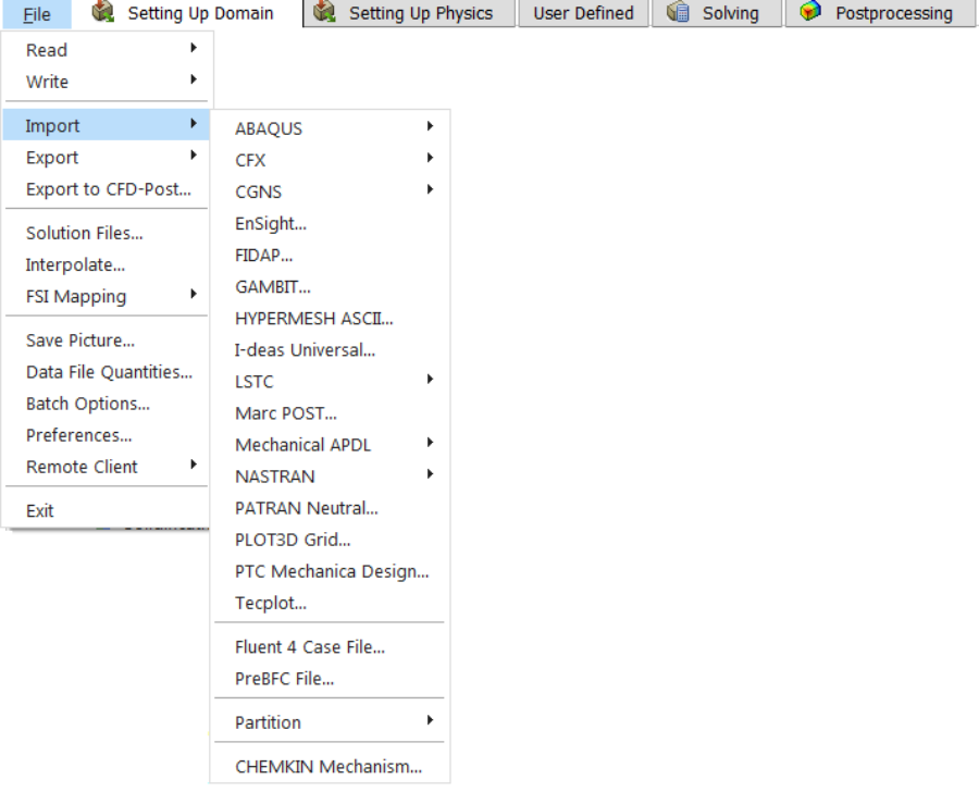
Import option in FLUENT
Import option in STAR-CCM+
For mapping temperature and pressure data to solvers like NASTRAN and ABAQUS: Export NASTRAN mesh as a *.BDF file or ABAQUS mesh as *.inp file and import it into STAR-CCM+ using "File->Import->Import CAE Model". Then use data mappers (available under Tools) to map the data to the NASTRAN mesh. Then export the data containing mapped nodal temperatures and pressures from STAR-CCM+ back onto the *.BDF format. Import it back into pre-processor say ABAQUS/CAE or Patran.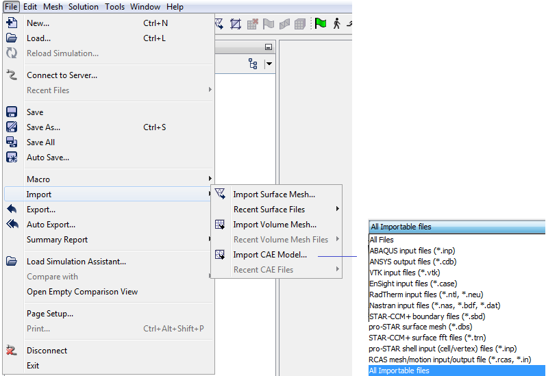
Post-Processing in CFD-Post
The variable temperature gradient is not available as standard. A derived variable can be created by selecting gradient operator and temperature as field variable. It will create 3 components named: "Temperature.Gradient X", "Temperature.Gradient Y" and "Temperature.Gradient Z". The names of expressions are sorted alphabetically in order A..Za...z. To export variables in CSV format in ANSYS CFD Post: File - Export - Export... and then under Options tab, set and choose (1) CSV File path and name, (2) Location (i.e. boundary locations) and (3) Variable(s). For vectors, select appropriate option under Formatting tab. Sync cameras: Views move together, Sync objects: Visibility of locations and plots is the same. In CFD-Post, the name of an expression or an object such as plane or contour cannot be changed once it has been created. To rename an existing object, create a duplicate with desired name and delete the original copy.If simulation results were created in FLUENT, reading *.cas and *.dat in CFD-Post have different behaviour. Since *.cas file contains only mesh and no result, reading *.cas file alone may not automatically load the correct result files. The *.dat file contains only the result (the variables at cell centers as FLUENT uses cell-centred scheme to create control volumes). Since it doesn't contain the mesh, loading only the *.dat file will not allow to create custom variable which may require interpolation to the faces and vertices of the cells. To combine both, FLUENT provides option to export the simulation data in .CDAT format.
The CFX State File (*.cst) created for one result file (*.res) cannot be used at it is for another result file with different zone (primitive boundary) names. The CST file contains the case name which needs to be updated. One roundabout option it to rename each case file to a "same unique name" on which *.cst file was created and saved.
CFX-Pre sometimes does not show surface mesh when selected. This seems to be a bug which can be overcome by running following session code.
> setPreferences User Import Executable = , Viewer Background Image File = , \
  Viewer Highlight Type = Wireframe
> update
> setPreferences Render Draw Faces = On
> update
> setPreferences Viewer Highlight Type = Surface Mesh
> update
> setPreferences Render Draw Faces = Off
> update
The polyline created by boundary intersection in CFD-Post sorts the point in ascending order along the axes. Hence, combining multiple polylines into a single polyline file using text editor needs to arrange the points such that they follow the sequence else extra (straight) polylines shall get created between the end point of one polyline and start point of next polyline because the are not same.
In a *.cst file, print all lines starting with string "CONTOUR"
$substr = "CONTOUR";
open(INFILE, "Case_123.cst");
while($line = <INFILE>) {
  $str = $line;
  # Convert the strings into lower case before comparing them
  if (index(lc ($str), lc($substr)) = -1) {
    if (index (1c($str), lc($substr)) == 0) {
      print "$str\n";
    }
  }
}
Solver variables are available for use in any expression: x, y, z: Direction 1, 2, 3 in Reference Coordinate Frame. r: Radial spatial location, r = (x^2+y^2)^0.5. theta: Angle, arctan(y/x). t: Time, u, v, w: Velocity in the x, y, z coordinate direction, p: (absolute) Static Pressure, ke: Turbulent kinetic energy, ed: Turbulent eddy dissipation, T: Temperature, sstrnr: Shear strain rate, density: Density, rNoDim: Non-dimensional radius (rotating frame only), viscosity: Dynamic Viscosity, Cp: Specific Heat Capacity at Constant Pressure, cond: Thermal Conductivity, AV name: Additional Variable name, mf: Mass Fraction
Post-process multiple *.res files either to compare or generate similar plots
cfd-online.com/Forums/cfx/91436-post-process-cfx.html: In CFD-Post, load all the files by checking the option "Keep current cases loaded" in the load results files window. As default option "Open in new view" is checked which creates a view for each case in one window. For each view you will be able to select time steps, set separate visualisation options and so on. To have all views with the same options there is a button called "Synchronize Visibility" which lets all vectors and contour plots appear in all views simultaneously. "Synchronize camera" enables the same angle of view and z0om factor in all views. Alternatively, load one file and open the "Load results" again, check "Keep current cases loaded" and uncheck "Open in new view" before second file is loaded. Then apply 'translation' on one of the cases to have two results in one view. Steps can be repeated for more files.Create separate meridional plots of the pressure side and suction side of a blade in CFD-Post: this is an important requirement if the suction and pressure side of blades are not split during pre-processing stage. innovationspace.ansys.com/.../how-to-create-separate-meridional-plots-of-the-pressure-side-and-suction-side-of-a-blade-in-cfd-post: this link provides a detailed explaination and sample CCL script.
How to hide all contours in CFD Post? This requires PERL subroutine getChildren which, as per CFX Reference Guide, returns the children of an object in a comma-separated list. Similar other utility 'getChildrenByCategory': to get a comma-separated list of all surfaces in a state at the top level (that is, not sub-objects of other objects): ! $surfaces = getChildrenByCategory("/", "surface");
! my @contour_list;
# 'split' converts the string into an array of strings
! @contour_list = split(",", getChildren("/", "CONTOUR"));
! foreach $contour (@contour_list) {
   # Sending visibility action from ViewUtilities
   > hide /$contour, view=/VIEW:View 1
! }
Function Calculator: CFD-Post has feature named "Function Calculator" for quantitative result generation. However, it allows to select only one boundary at a time. Create surface group of boundaries to select more than one boundary at a time (use shift+control while clicking on the zone or domain names to select multiple domains and all the boundaries defined for that domain). The function calculator has two additional options: "Show equivalent expression" - which will print CCL expression for the GUI version and "Clear previous results on calculate" - which should be turned-off to keep all results in the output window.
Post-processing for Turbo-machines
The post-processing activities of turbomachines require understanding of special terms like Turbo surface, Meridional plots, Span Normalized, ACA: Area Circumferential Average, LCA: Line Circumferential Average, Blade Aligned Edge... CFD-Post has Turbo mode with special features not available in outline mode. Promote to General Mode: this method can be used to copy the selected plot object and any required supporting objects (for example, a line locator) to the Outline workspace. This would enable, for example, the selected plot to be included in a report. Under Turbo tab in CFD-Post, Calculate Velocity Components creates a variable called Velocity Circumferential which is the swirl velocity.
For post-processing of turbomachines in STAR-CCM+ refer to the tutorial "Gas Turbine Aerodynamics" which explains how to generate meridional and streamwise plots.The Blade-to-Blade and Meridional objects can be copied into the Outline tree view by right-clicking and selecting Promote to General Mode. "Span Normalized" defines the dimensionless distance (between 0 and 1) from the hub to the shroud. The Blade-to-Blade object is used to view plots on a surface of constant span. The Meridional object is used to view plots on an axial-radial plane. A surface of constant Theta at 0 degrees is created. In turbo line, turbo surface, and related editors, the Blade Aligned coordinate values entered in the input fields (and the related CCL parameters) are normalized to the leading and trailing edge locations of blade with predefined constant references: 0.25 and 0.75 are taken to be the blades leading and trailing edges, respectively. Note that Meridional Surface is a reserved name in CFD-Post.
The main purpose of Turbo mode is to make the ACA (Area Circumferential Average) value of field variables available for Outline Mode. Thus, once a contour in Turbo Mode under Plots -> Meridional, is generated say for Pressure, a location named "Meridional Surface" and a variable "Pressure ACA of Meridional Surface" become available in Outline Mode for generation of contour plots. Similarly, a contour plot of "Velocity Meridional" shall make a variable "Velocity Meridional ACA on Meridional Surface" available in Outline Mode. Velocity Meridional itself ia available only when "Calculate Velocity Components" under Turbo mode is executed. This operation creates many other variables such as Velocity Axial, Velocity Blade to Blade, Velocity Circumferential, Velocity Radial, Velocity Spanwise, Velocity Streamwise, and X- Y- Z-Components of "Velocity Meridional" & "Velocity Blade to Blade".Many a time the background mesh generation of meridional plane fails for one of the domains. One of the options is manual initialization by selecting hub option to "From Line" instead of default value of "From Turbo Regions". Before that a polyline representing hub needs to be created using "Boundary Intersection" method. This is a trial and error approach though and different polylines would need to be tried out. Note that many a time, the domain comprise of 3 sub-domains, stationary one upstream the rotation blade domain and another stationary sub-domain downstream. The definition of hub and shroud should be connected walls used to define the hub and shroud for rotating domains.
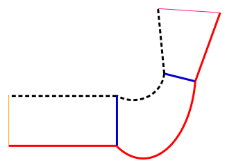
In the image above, the red lines should be defined as hub to respective zones and dottend lines as shrouds.
Centre of Pressure
Centre of pressure - CofP (which depends on the location of each cell and pressure force acting on it) is not same as coefficient of pressure - Cp (which depends on the total pressure force and a arbitrarily chosen reference area). The center of pressure is the point on a body where the total sum of a pressure field acts, causing a force and no moment about that point.
CofP = ∫(x * P.dA)/∫(P.dA) or discretely as ∑(xi * π *Ai)/∑(π * Ai), Cp = ∫(P dA) / AREF
Force-Momentum equation about origin:- Let {F} = (Fx, Fy, Fz) and {M} = (Mx, My, Mz)
- Mx = 0*x + Fz*y - Fy*z
- My = -Fz*x + 0 *y + Fx*z
- Mz = Fy*x - Fx*y + 0*z
- As diagonal of the [F] matrix in {M} = [F] {x} is zero, they are singular (i.e. one or more equations are not independent). inv(F) does not exist and det[F] = 0.
- Unit vector in force direction {f} = {F}/|F| = (Fx, Fy, Fz)/|F| where |F| = sqrt(Fx*Fx + Fy*Fy + Fz*Fz)
- Moment parallel to F (pure couple) can be calculated by taking component of {M} along {f}. Thus: {MF} = [{M}.{F}] {f} = (Fx, Fy, Fz) * (Mx*Fx + My*Fy + Mz*Fz) / |F| / |F|
- We need to find a location about which Mz = 0 then using the equations Mz = Fy*x - Fx*y + 0*z we get 0 = Fx*x - Fy*y. Thus, y = (Fx*x)/Fy
- Mz = -Fx *y + Fy * x and y = (Fx*x)/Fy. Thus: Mz = -Fx*(Fx*x)/Fy) + Fy*x = (-Fx2/Fy)*x + Fy*x
- Hence, x = Mz/(-Fx2/Fy + Fy)
- Note: The equations used to calculate the CofP location cannot be used to calculate the moment at the CofP. The moments in those equations are the moments about the origin.
Rules of Thumb: Interpolation of Results
Observations and Design Recommendations
The reports must contain a section with observations, conclusion from simulation and recommendations for further actions. Note that the target recipient of simulation reports may be design engineers which may or may not be familiar with reading plots and graphs.- Explain the meaning of your observations in relation to the simulation objectives and real-world implications
- Provide key insights by highlighting the most important findings from the simulation, including potential strengths and weak areas of the system being investigated
- Based on result analysis and insight gained, propose actionable steps or design changes to improve the system performance or meet permissible limits.
- If appropriate, present the validity of simulation results and identify potential limitations of the model and boundary conditions used.
- Example from "PLM Thermal Analysis Report" document number ARIEL-INAF-TN-0003:
- The thermal model results, heat fluxes across the interfaces and units temperature, indicate a reliable PLM thermal architecture, compliant to the requirement including the present level of margin. The next steps of the thermal analysis will be aimed to reach a higher level of detail, to optimize the design and to prepare a more reliable assessment of uncertainties and margins at the interfaces.
- For both thermal cases, all temperatures result below, or at, the required values including margin, indicating a fully compliant thermal architecture with some extra space for further optimizations. In phase B1 the thermal architecture will be optimized to reduce the uncertainty margins and increase the design margins on the passive and active cooling stages, especially the coldest ones.
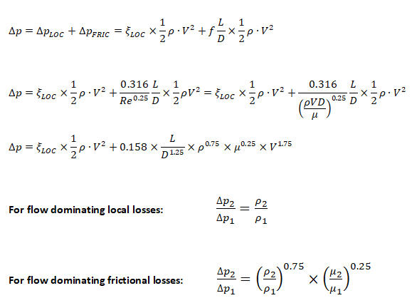
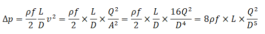
One of the expectations from a simulation engineer is to provide design recommendations that may help those who are not familiar with fluid mechanics and heat transfer or those who may not be able to interpret the contour plots. For example, if pressure drop criteria is not reached, one recommendation would be to increase the width of the flow channels. But this is only an opinion and cannot be classified as design recommendations. "Increase the diameter by 20% and increase the ratio of bend radii to tube diameter to value ≥ 2.0" is a design recommendation easier to follow and implement. In order to arrive at these numbers, one has to be familiar with the empirical correlations and thumb-rules. For example, the dependence of pressure drop on diameter of circular channels and gap of narrow channels are described below.
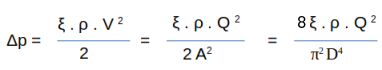
For circular, squre or nearly circular channels
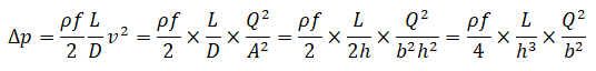
For rectangular channels
Following short calculator can be used to estimate diameter to achieve desired pressure drop - use consistent units for diameter and pressure drop, units mentioned here are for reference only.
| Specify hyd. dia. of baseline orifice: | [mm] | |
| Specify number of parallel orifices: | [-] | |
| Specify calculated / measured pressure drop: | [Pa] | |
| Specify desired pressure drop: | [Pa] | |
| Specify desired number of orifices: | [Pa] | |
| Click on submit button to calculate new diameter | ||
| n | 6 | 8 | 10 | 12 | 16 | 20 | 25 | 32 | 50 |
| Area ratio: | 0.8270 | 0.9003 | 0.9355 | 0.9549 | 0.9745 | 0.9836 | 0.9895 | 0.9936 | 0.9974 |
Post-processing for DPM
When tracking particles in parallel, the DPM model cannot be used with any of the multiphase flow models (VOF, mixture, or Eulerian) if the Shared Memory option is enabled.
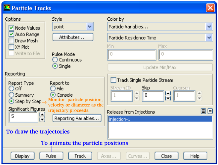
ANSYS FLUENT reports the magnitudes of the interphase exchange of momentum, heat, and mass in each control volume as well as the total concentration of the discrete phase. These variables can be displayed graphically, by drawing contours or profiles and are available under the Discrete Phase Model... category of the variable selection drop-down list in post-processing dialogue boxes.
Particle states (position, velocity, diameter, temperature, and mass flow rate) can be written to files at various boundaries and planes (lines in 2D) using the Sample Trajectories Dialog Box accessed by Reports -> Sample -> Set Up... Histograms can be plotted from sample files created in previous step by Reports -> Histogram -> Set Up...
Trajectory Fates: Shed trajectories are newly generated particles during the breakup of a larger droplet and appear only if a breakup model is enabled. Coalesced trajectories are removed particles which have coalesced after particle-particle collisions and appear only if the coalescence model is enabled. Splashed trajectories are particles which are newly generated when a particle touches a wall-film. Those trajectories appear only if the wall-film model is enabled.
Post-processing for Radiation
In STAR-CCM+ one can calculate the radiation view factor for S2S model using solver tree as shown below. The view factor summary can also be printed using option "Display View Factor Summary".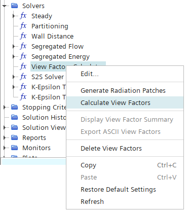
Post-processing for Transient Runs
Time statistic information is available under "Unsteady Statistics" in post-processing such as Contours, Surface integrals... It provides two kinds of statistics: mean and root-mean-square (RMS) of the chosen field variables and custom field function. ANSYS Fluent applies a simple averaging process to calculate mean and hence the accuracy of the numerical integration is limited to that of a basic rectangle method. This is reasonably accurate unless the time gradient is too high or time steps are large.The energy balance for transient runs is tricky in the sense one cannot balance heat transfer rates at any instantaneous value. This is because of change in internal energy in the system. /report/volume-integrals mass-integral (*) internal-energy no: this TUI command calculated internal-energy of solids and fluid zones in unit [(J/kg)(kg/m^3)(m^3)] which is nothing but [J]. Note that this value alone has no meaningful physical significant (and can be negative as well). This computation should be done at start of the simulation and any other time of interest. The difference between two values shall be the change in internal energy that can be used to check for energy balance.
Overall Checklist
| No. | Checkpoint | Record [Y/N] |
| 01 | Have the fluid and solid zones named as per material type say by adding air, ss, al, pl, cr (ceramics)... as suffix? | |
| 02 | Have appropriate prefixes been added to the boundary names as per boundary type: e.g. mf for mass-flow, vi for velocity inlets, po for pressure outlets... | |
| 03 | Has the mesh quality been checked for skewness and aspect ratios (for boundary layers and for freestream elements)? | |
| 04 | Have sliver elements been collapsed? With minimum size ~ 0.05 [mm], elements having area < 0.002 [mm2] or volume 0.0001 [mm3] are unreasonable. | |
| 05 | Have the areas of the boundaries been checked and matched with the values used to estimate boundary condition parameters? | |
| 06 | Have the walls been grouped into logical surface-groups easy to maintain during solution and post-processing? | |
| 07 | Have the inlet and outlet planes of a porous domain been assigned to separate internal patches? | |
| 08 | Has the basic checks been made: scale of mesh, quality, default interfaces settings (CFX may create unwanted interfaces)? | |
| 09 | Has the density, viscosity and thermal conductivity of fluid been correctly assigned as per operating temperature and pressure? | |
| 10 | Has the auto-save frequency and file name correctly defined? For runs on clusters, specify only file name without full path. | |
| 11 | For transient simulations, have the specific heat capacity and density of solids been correctly assigned? | |
| 12 | Has the relaxation factors for k, ε and turbulent viscosity been reduced to value lower than 1.0 say 0.25 or 0.50? | |
| 13 | Has the convergence criteria been set to low value such as 1e-05 or lesser? Run may stop early if set to higher number such as 1e-3. | |
| 14 | Has the discretization schemes set to first order for initial 500~1000 iterations? Gradually move to second order. | |
| 15 | Has the monitor points been created for global mass imbalance? | |
| 16 | In FLUENT, have contour plots been created? This helps avoid repeating the process on repeated set-up of different cases. | |
| 17 | Has a monitor for heat transfer through all walls been created? Do not include inlets and outlets. | |
| 18 | Have the interfaces of porous and fluid domains changed to type 'internal'? |
Overall Steps of Simulations
The following table summarizes all the steps which one needs to follow to make CFD simulations. They have already been described in detail on various pages of this website. Yet, the following table shall act as a ready-reckoner for the information to look for.
| Step | Description of the Step | Activities Performed | Tool Name |
| 01 | Prepare the geometry | Rename the parts as per identifier such as applicable boundary condition, material or interface type. Check for symmetry and need to domain extension especially at outlet(s). | SpaceClaim, HM, ANSA |
| 02 | Inspect geometry | Check for interferences, gaps, proximities and leakages to ensure volumes do not mix and merge | SpaceClaim, HM, ANSA |
| 03 | Create named selection or names zones / patches | To apply required mesh setting and boundary conditions - easy to filter and select in subsequent operations | SpaceClaim, HM, ANSA |
| 04 | Prepare geometry for pre-processor | Split bodies, Merge volumes, imprint surfaces, share topology (merge overlapping surfaces) | SpaceClaim, ANSA, HM |
| 05 | Import the CAD geometry in pre-processor (meshing) | Get boundary mesh and required refinement at curvatures | FLUENT Mesher, ANSA, HM |
| 06 | Correct surface mesh for topological and quality issues | Intersections, proximities, leakages, skewed cells, high aspect ratio (sliver elements) | FLUENT Mesher, ANSA, HM |
| 07 | Define meshing parameters | Global mesh controls, local mesh controls, boundary layer controls | FLUENT Mesher, ANSA, HM |
| 08 | Compute volume | Regenerate volumes for fluid and solid zones, ensure each volume is correctly identified | FLUENT Mesher, ANSA, HM |
| 09 | Generate volume mesh | Check quality of volume mesh: skewness (≤ 0.90), orthogonality (≥ 0.10) and aspect ratio (≤ 50) | FLUENT Mesher |
| 10 | Improve mesh quality | Use mesh improvement tools (move and merge nodes, refine mesh) to meet required target | FLUENT Mesher |
| 11 | Export mesh into solver format and read into pre-processor | Check the mesh, scale into metric units | FLUENT Pre-Post |
| 12 | Apply solver settings | Define materials, boundary conditions, turbulence models, relaxation factors | FLUENT Pre-Post |
| 13 | Identify run-time variables | Define monitor points and planes, section planes for contours, result back-up frequency | FLUENT Pre-Post |
| 14 | Make runs | Monitor convergence residuals | FLUENT Solver and Cluster |
| 15 | Post-process result | Create contour plots, vector plots, streamlines, animations | FLUENT Pre-Post, CFD-Post, ParaView |
| 16 | Create special plots | Overlap of contour and vectors, Iso-volumes, Import special planes for post-processing, uniformly spaced vectors | FLUENT Pre-Post, CFD-Post, ParaView |
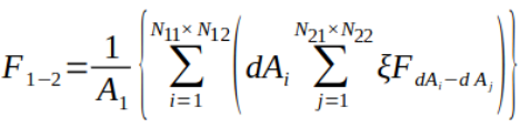
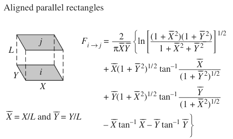
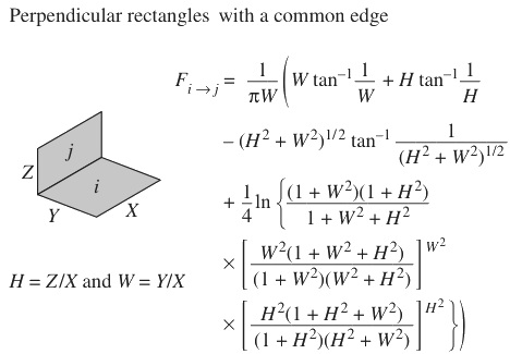
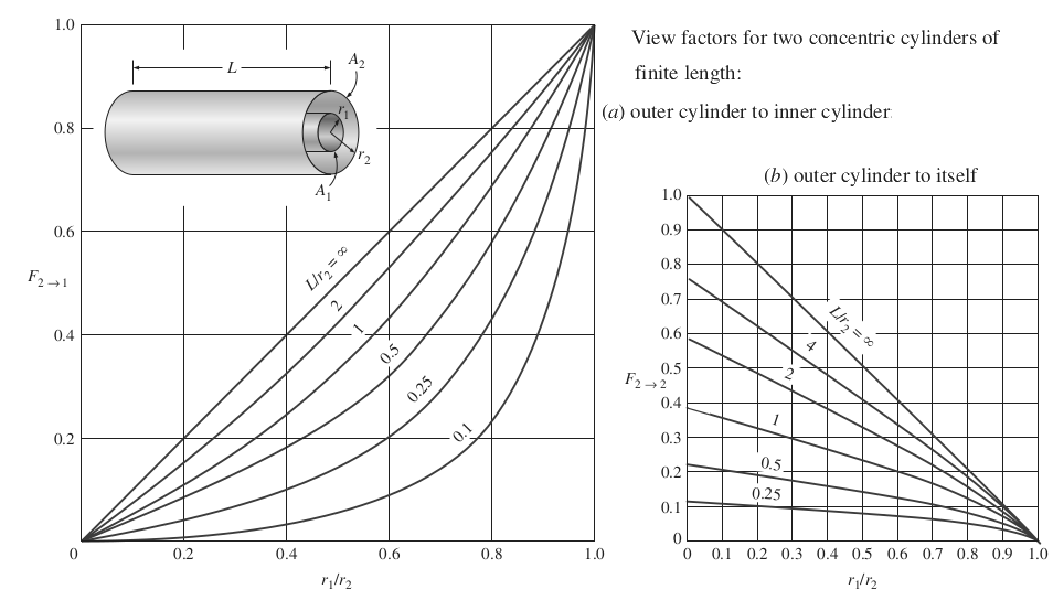
Radiation View Factor and Other Equations
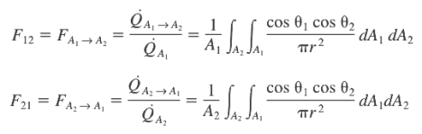
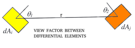
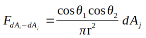
Radiation View Factor for Concentric Spheres
Radiating heat transfer rate from inner sphere is given by following equation. Note that the view factor of inner sphere to outer sphere is 1.0 as all radiation leaving inner sphere is trapped by the outer one.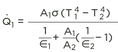
| Ratio of Radii | 0.050 | 0.100 | 0.200 | 0.300 | 0.400 | 0.500 | 0.600 | 0.700 | 0.800 | 0.900 | 0.950 | 0.975 |
| FOUT_IN | 0.9975 | 0.9900 | 0.9600 | 0.9100 | 0.8400 | 0.7500 | 0.6400 | 0.5100 | 0.3600 | 0.1900 | 0.0975 | 0.0494 |
| Ratio of Radii | 0.150 | 0.250 | 0.350 | 0.425 | 0.450 | 0.550 | 0.650 | 0.750 | 0.850 | 0.875 | 0.925 | 0.985 |
| FOUT_IN | 0.9775 | 0.9375 | 0.8775 | 0.8194 | 0.7975 | 0.6975 | 0.5775 | 0.4375 | 0.2775 | 0.2344 | 0.1444 | 0.0298 |
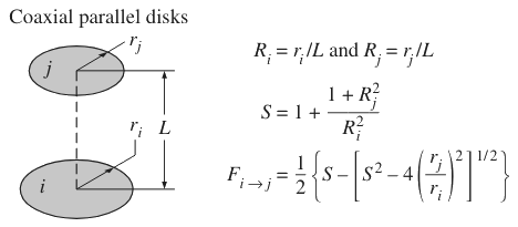
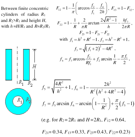
Few very special configurations such as "Ground plane to the outer surface of a cylinder (radius r2, height h) at a distance L above a ground plane (a planar disk of radius r1)" and their few factors are described in "HLS-UG-001: BASELINE RELEASE - "HUMAN LANDING SYSTEM LUNAR THERMAL ANALYSIS GUIDEBOOK" published by NASA. Some other configurations are: Outer surface of a cylinder (radius r1, height h) to the ground plane (a planar disk of radius r2), Outer surface of a sphere located at a distance h above the ground plane to the ground plane (a planar disk of radius r2), Outer surface of a hemisphere (radius r1) to the ground plane (a planar annular disk of radius r2), Outer surface of a “small” sphere (radius r1) to a "much larger" sphere (radius r2) where the centers of the two spheres are separated by a distance h.
Template of Report
It is better to start recording the information to be put in a report from the start rather than preparing the report at the end of the simulation activity.PAGE-01:
Scope: carry out a steady-state, single-phase, incompressible, forced-convection, passive cooling with radiation... simulation for product/assembly.
Objective: The intent of this simulation to estimate pressure-drop, hot-spot, stagnation zones... and compare with provided design limits.Expected deliverables: a short simulation report in PowerPoint or Word format with go/no-go decisions and design recommendations to improve the performance or meet the specifications.
Add picture of the project (isometric view) alogn with some sectional view(s) which provide most information about shape and look.PAGE-02:
Computational Domain and Boundary Conditions: Use section images and highlight important boundaries: inlet, outlet, heat sources, fans, porous domains...PAGE-03:
Assumptions and Approach: add methods used to arrive at boundary conditions, justifications for domain size reduction or extension, material selection and source of material properties.PAGE-04:
Mesh statistics and key solver settings: Mention the type of mesh (tetrahedral with 3 prism layers, polyhedral...), total number of surface elements, total number of volume elements, maximum aspect ratio and worst skewness (optionally number or % of cells with skewness > 0.95).PAGE-05:
Result Summary, Key Observations: This slide should present bulleted or tabulated data extracted from simulations such as pressure drop, number of parts not meeting temperature limit criteria...PAGE-06:
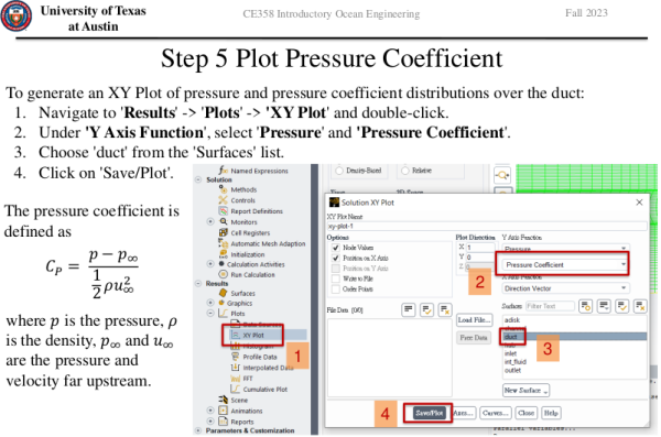
Contour / Vector / Steamline Plots: add an image showing the location of section and viewing direction (which sometime may be omitted if axes triad are clearly visible). On each plot, add 1-2 statements of summary, the recipients of the report may not be simulation engineers and not all eyes are trained to interpret plots. For example:"This is the pressure distribution plot in a section aligned with XY-plane and passing through the axis of inlet boundary. The colour-bands indicate the variation of pressure values in the plane and important is to note the sharp gradient near the elbow bend where flow separates."
"This is a surface temperature plots for all parts mounted on the PCB and the locations with red color indicate the highest temperature calculated. The blue regions are the the colder zones of the assembly with 10 [°C] rise over ambient condition."
PAGE-NN:
Recommendations: This slide should give reference to previous slides which giving more insight into the simulation results and why the suggestions put forward are likely to work. Example: "As can be viewed on zone encircled on slide M, the high temperature of part X is affecting the temperature of nearby parts. To bring the temperature down for this zone, either the distance between the parts need to be increased or this high heat density part should be moved to other location or provided with a heat spreader."A section named "Observations" can also be added with following content. "Good convergence obtained for all field variables except continuity which can be attributed to reverse flow at outlet and less than optimal mesh refinements in recirculation regions." No regions of excessive temperature gradient observed indicating all thermal contacts are perfectly captured. High temperature in a narrow region neat part X indicate relatively poor conduction path. The area near part Y has uneven temperature distribution indicating potential draft and/or inefficient heating/cooling.
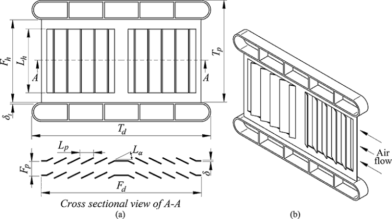
For example: one may ask how the louvred fins increase overall heat transfer rate when the slit in geometry breaks the conduction path and increases overall pressure drop? Reference article "Heat Transfer Enhancement by Perforated and Louvred Fin Heat Exchangers" by Miftah et. al.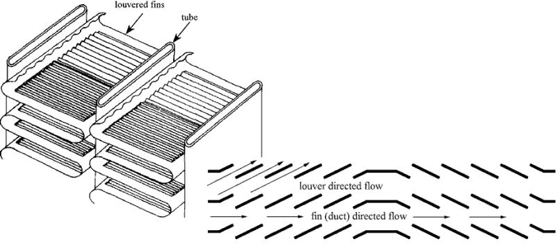
Heat Conduction through Wires
The content on CFDyna.com is being constantly refined and improvised with on-the-job experience, testing, and training. Examples might be simplified to improve insight into the physics and basic understanding. Linked pages, articles, references, and examples are constantly reviewed to reduce errors, but we cannot warrant full correctness of all the contents.
Template by OS Templates