Extended Surfaces and Heat Spreaders

Heat Transfer in Straight Fins

Fins as extended surfaces have wide applications in heat transfer augmentation techniques. The solutions are already available in analytical form. Refer to this PDF file for MathCAD calculations for fins.

The OCTAVE script below tries to prepare a plug-and-calculate method for straight fins for all possible combinations of boundary conditions.

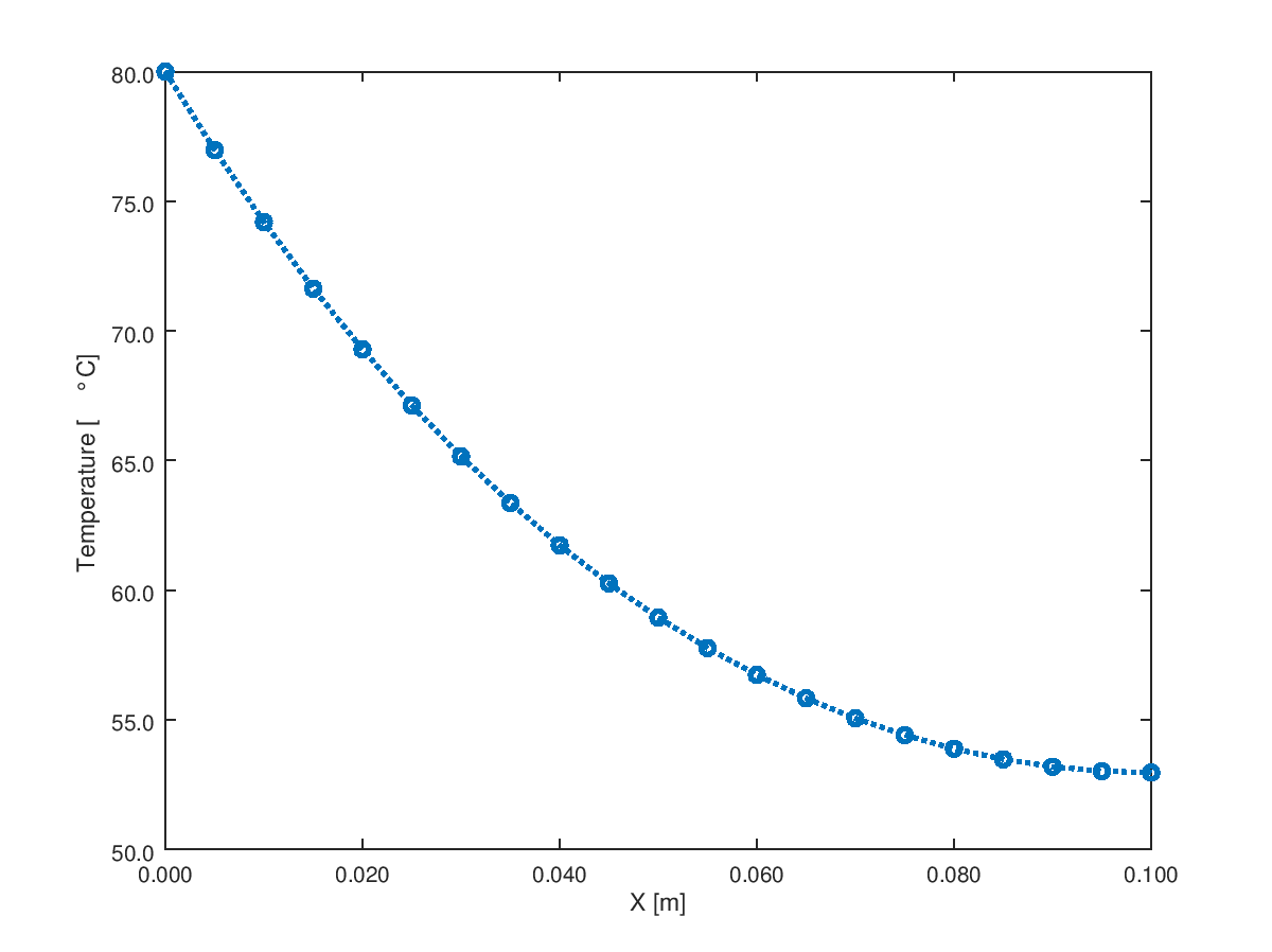
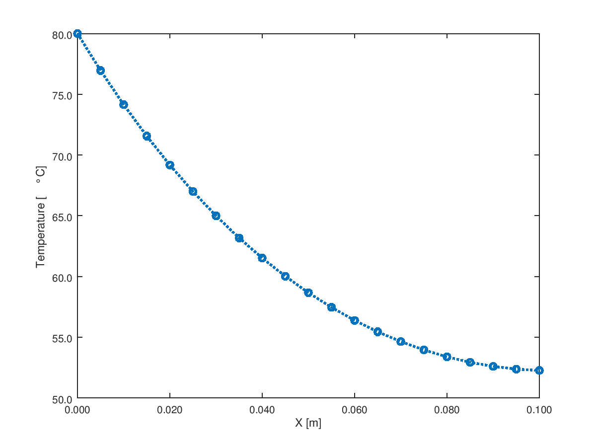
Temperature Plots

Note that the heat transfer at base is 9.867 [W]. This value can be used to calculate temperature profile T(x) for "Heat Flux" (base) - Adiabatic (tip) boundaries to ensure that the temperature at base is same as in previous case. This is sort of the quality assurance (QA) method for the code and not the analytical methods described in the textbooks on heat transfer.

% Fin performance calculation for all possible boundary conditions
% 
  clear; clc;
% Thermal conductivity of fin material in [W/m.K]
  k = 200;
%
% Convective heat transfer coefficient over fin surface in [W/m^2.K]
  h = 100;
  TREF = 30; 
%
% Perimeter of the fin [m]
  p = pi*0.01;
%
% Cross-section area of the fin [m^2]
  A = pi/4*0.01^2;
%
% Length of the fin in [m]
  L = 0.10;
%  
% Boundary condition at base: 1 - Known temperature [C] - T0 
%                             2 - Heat flux [W/m^2] - Q0
%
  BC1      = 1;
  valueBC1 = 80; %9.8675/A;
%
% Boundary condition at Tip: 1 - Known temperature [K], 
%                            2 - Known heat flux [W/m^2] (< 0 if heat loss)
%                            3 - Convection, h_tip = h [W/m^2-K], TREF2 = TREF
% Note that "positive value" of heat flux is heat flow into the fin body.
  BC2      = 3;
  valueBC2 = h;   % TL or QL or hTip 
  
%
% Number of calculation points [recommended to be an odd integer]
  n = 21;         

% -------------User Input Ends ------------------------------------------------
%---------------------+------------------+------------------+------------------  

  x = [0 : L/(n-1): L];
  m = sqrt(h * p / k / A);
  b = sqrt(h * p * k * A);
  T = zeros(n);
  if (BC1 == 1)
    if (BC2 == 1)
	   Tr = (valueBC2 - TREF) / (valueBC1 - TREF);
       Tx  = TREF + (valueBC1 - TREF) .*  (sinh(m .*(L - x)) ./ sinh(m .* L) ...
	               +  Tr .* sinh(m .* x) ./ sinh(m .*L));
       Q0 = b * (valueBC1 - TREF) * (1 / tanh(m * L) - Tr / sinh(m * L))
       QL = -b * (valueBC1 - TREF) * (1 / sinh(m * L) - Tr / tanh(m * L))
 	   T0 = valueBC1
	   TL = valueBC2
%
    elseif (BC2 == 2)
	   qL = valueBC2 / k / m;
	   q0 = valueBC1 - TREF;
       Tx = TREF - (qL + q0 .* sinh(m .* L)) ./ cosh(m .* L) .* sinh(m .* x) ...
	             +  q0 .*  cosh(m .* x);	
       Q0 = b * (qL + q0 * sinh(m * L)) / cosh(m * L)
	   QL = valueBC2 * A
	   T0 = valueBC1
	   TL = Tx(end)
%	   
    elseif (BC2 == 3)
	   hr = valueBC2 / k / m;
       Tx =  TREF + (valueBC1 - TREF) .* (cosh(m .* x) - (hr + tanh(m .* L)) ...
	            ./ (1 + hr .* tanh(m .* L)) .* sinh(m .* x)); 	
       Q0 = b * (valueBC1 - TREF) * (hr + tanh(m * L))/ (1 + hr * tanh(m * L))
	   QL = -valueBC2 * A * (Tx(end) - TREF)
	   T0 = valueBC1
	   TL = Tx(end)
	end
  end
%  
  if (BC1 == 2)
    if (BC2 == 1)
	   Qr = valueBC1 / k / m;
	   Tx = TREF - Qr .*  (sinh(m .* x)) + ((valueBC2 - TREF)+ Qr .*  ...
	               sinh(m .* L)) .* cosh(m .* x) ./ cosh(m .* L);
       Q0 = valueBC1 * A
       QL = -b * (Qr * cosh( m * L) - ((valueBC2 - TREF) + Qr * ...
	             sinh(m * L)) * tanh(m * L))
	   T0 = Tx(1)
	   TL = valueBC2
%	   
    elseif (BC2 == 2)
	   Qr = valueBC2 / valueBC1;
       Tx = TREF + (valueBC1 .* A ./ b) .*  (cosh(m .* (L - x)) ...
	             ./ sinh(m .* L) + Qr ./ tanh(m * L));	
       Q0 = A * valueBC1
	   QL = A * valueBC2
	   T0 = Tx(1)
	   TL = Tx(end)
%	   
	elseif (BC2 == 3)
	   hr = valueBC2 / k / m;
	   qT = valueBC1 / k / m;
       Tx = TREF - qT .* sinh(m .* x) + qT .* (1 + hr .* tanh(m .* L)) ...
	            ./ (hr + tanh(m .* L)) .* cosh(m .* x);
	   Q0 = valueBC1 * A		
       QL = -valueBC2 * A * (Tx(end) - TREF)
	   T0 = Tx(1)
	   TL = Tx(end)
	end
%	
  end 
% Plot temperature profile
  plot(x, Tx, "linestyle", ":", "linewidth", 2, "marker", "o");
  xlabel('X [m]'); ylabel('Temperature [\degC]');
%  
  % Format X-axis ticks
  xtick = get (gca, "xtick"); 
  xticklabel = strsplit (sprintf ("%.3f\n", xtick), "\n", true);
  set (gca, "xticklabel", xticklabel)   
%  
  % Format Y-Axis ticks
  ytick = get (gca, "ytick"); 
  yticklabel = strsplit (sprintf ("%.1f\n", ytick), "\n", true); 
  set (gca, "yticklabel", yticklabel);
%
  print -dpng finTempAdiab.png -color -landscape;
return