- CFD, Fluid Flow, FEA, Heat/Mass Transfer: FEEDBACKS/QUERIES -

BOUNDARY CONDITIONS
Boundary Conditions: Last Updated on 24-Feb-2024
Type of Boundary Conditions, Applications and Limitations
What is physical and mathematical significance of a boundary condition?
The boundary conditions of any problem is used to define the upper and lower limits of the field variables at the boundaries. These are the operating conditions which govern both the micro- and macro behaviours of these variables. A suitable choice of boundary conditions is as good as a good test set-up! Intuitively, a boundary condition implies that "it is known what happens" on a particular boundary.
When comparative studies are performed, choice of boundary conditions becomes even more important. For example, if the performance of plain fin and louvred fin designs are to be compared, the inlet velocity boundary condition is not appropriate as it does not account for different pressure drops. The appropriate boundary conditions would be pressure inlet and pressure outlet boundary conditions imposing equal pressure drops in the two systems. A counter argument can be that the fixed pressure drop boundary conditions does not account for different flow velocities. Hence, the final decision should be based on system performance. If the heat exchanger is dominant contributor (> 80%) to system resistance, the pressure drop boundary conditions would be more appropriate. On the other hand, if heat exchanger is the minor contributor (< 20%) to system resistance, the inlet velocity boundary conditions would be more appropriate as flow rate through the system shall not change significantly.
Table of Contents: POROUS Boundary Conditions | Interpolation of Results | Wall Boundary Conditions for DPM and Radiation | Heat Exchanger Modelling | Multiphase Flows | License Manager: LMTOOLS | Volumetric Heat Sources | Periodic Boundary Conditions | Unit Conversion | Rotating Domains | Text User Interface (TUI) in FLUENT | Checklist for Inputs of Boundary Conditions | Symmetry Boundary Conditions | Centre of 3 points | Unit Vector between 2 Points | Porous Loss Coefficient Calculator | Binary Diffusion Coefficients |*| Material Properties of Moist Air |-| Fan Boundary Conditions |:| Real Gas Properties
Heat Source and Material Properties as Tabulated Data |+| Equivalent Orthotropic Thermal Conductivity
For flow and thermal simulation jobs, consultancy, training, automation and longer duration projects, reach me at  . Our bill rate is INR 1,200/hour (INR 9,600/day) with minimum billing of 1 day. All simulations shall be carried out using Open-source Tools including documentations.
There are different (combination) of boundary conditions. For example, in a structural simulation, the number of boundary conditions can be varied to ensure the force- and moment balance of the entire system. This can be achieved by applying boundary condition at just one node or at 6 different nodes! Similarly, in any fluid problem, there must be an entry and an exit for the fluid (as an exception buoyancy-driven flow can be omitted for the time being). This most basic condition is termed as "Inlet" and "Outlet" boundary conditions in CFD parlance, though the choice of "field variables" such as velocity, pressure, temperature, mass flow rate, may vary as per problem set-up.
Naming Convection of Boundaries and Cell Zones
In any practical application of CFD simulations, the computational domain may comprise of many cells zones (fluid and solid zones) and boundary zones (walls, inlets and outlets). The engineer responsible for pre-processing may not be the one who creates solver file and post-processes the results. The reviewer(s) of the mesh and simulation set-up will certainly be not the engineer who created them. In order to convey the domain information seamlessly, a naming convention should be adopted, it can be a generic system applicable for large number of projects or a specific system for particular simulation set-up. An example is outlined below with following default setting: Newtonian, stationary, adiabatic, smooth boundaries or zones can be named arbitrarily though it is recommended to chose names and identifiers meaningfully. Note that some programs assigns appropriate boundary conditions based on the keywords present in the zone names such as Inlet, Outlet, Periodic, Interface, Hub, Shroud, Blade, Wall...
- Inlet(s) and outlet(s) should be named as b_inlet_id, b_outlet_id where 'id' stands for identifier.
- Walls with boundary conditions (other than adiabatic): w_tpr_id, w_hfx_id, w_htc_id, w_rot_id w_mov_id, w_rgh_id, w_s2s_id where 'rgh' stands for rough walls, s2s stands for coupled solid walls.
- Cell zones: fld_air_id, fld_wtr_id, fld_oil_id, fld_nnw_id, fld_rot_id, por_mom_id, por_thm_id, sld_alm_id, sld_stl_id, sld_src_id ... where 'nnw' stands for non-Newtonian fluids, 'src' stands for solid zones with heat source and/or sink and 'por' stands for porous (fluid) zones.
- Internal planes: int_f2f_id, int_baf_id ... where 'baf' stands for thin walls or baffles.
- Non-conformal interfaces: if_f2f_id, if_s2s_id, if_sta_rot_id, if_por_fld_id, if_por_por_id where 'sta' stands for 'stationary' zones and 'por' stands for 'porous' zones.
- All boundaries with no special setting or conditions to be applied on them can be named as 'b_def_id' or dumy-id1, dumy-id2 or empt-id1, empt-id2 or fblk-id1, fblk-id2 where dumy stands for dummy, empt for empty and fblk for flow-blockers. This is especially important while dealing with assemblies with large number of solids and fluid zones.
Material Properties
References - [1]: "Fluid Mechanics, Fourth Edition, Frank M. White", [2]: "HEAT AND MASS TRANSFER by YUNUS A. ÇENGEL from University of Nevada and AFSHIN J. GHAJAR from Oklahoma State University", [3]: "Handbook of Hydraulic Resistance by I. E. Idelchik", [4]: "Chemical and Process Thermodynamics by B. G. Kyle", [5]A Heat Transfer Textbook, Fifth Edition by John H. Lienhard IV and John H. Lienhard V
Conversion Factors as per Reference [1] - Mass and Volume: 1 slug ≡ lbf.s2/ft = 32.174 lbm = 14.594 kg, 1 lbm = 0.4536 kg, 1 U.S. gal = 0.0037854 m3, 1 U.S. fluid ounce = 2.9574E-5 m3, 1 lbm/ft3 = 16.0185 kg/m3, Pressure and Viscosity: 1 lbf/ft2 = 47.88 Pa, 1 poise = 1 g/cm.s = 0.1 Pa.s, 1 slug/ft-s = 47.88 Pa.s, Force and Energy: 1 lbf = 0.4536 [kg]*9.80665[m/s2] = 4.4483 [N], 1 BTU = 252 cal = 1055.056 J, 1 cal = 4.1868 J. Sometimes LFM (Linear Feet per Minute) is used to refer flow velocity - similar to the concept of CFM.
Other units: Specific Heat: 1 Btu/lb-°R ≡ 1 Btu/lb-°F= 4186.8 J/kg-K, Thermal Conductivity: 1 Btu/h-ft-°R = 1.7307 W/m-K Derived units: 1 BTUH = 0.29307 W, 1 gal/min or GPM = 0.06309 L/s, 1 CFM or ft3/minute = 4.72E-4 m3/s = 0.472 L/s Power: 1 ft-lb/minute = 2.2597E-2 [W]. 1 BTU/hr = 0.29307 [W], 1 BTU/hr/in3 = 0.29307[W]/[0.0254 m]3 = 17884.3 W/m3. Conversion method: 1 (BTU/h)/in/R = 0.29307 [W] / 0.0254 [m] / (5/9) [K]= 20.769 W/m-K -replace each unit on the left with equivalent value in other unit on the right taking care of numerator and denominator.
Validity of Continuum: It is assumed that the underlying assumption of continuum is valid for fluids. The assumptions of continuum breaks down at very low pressures and molecular dynamics takes over. Thus, application of CFD simulations to fluids under vacuum conditions should be taken after calculating Mean Free Path length which is calculate as λ = 1/[π√2] x 1/[d2NA] x R.T/p where d is the diameter [m] of the gas molecule, NA is the Avogadro number, R is the specific gas constant [J/kg-K], T is temperature of gas in [K] and p is absolute pressure in [Pa]. A dimensionless parameter Knudsen number, Kn = λ / L, where λ / L, where λ is the mean free path and L is the characteristic length describes the degree of departure from continuum. Usually when Kn ≥ 0.01, the concept of continuum does not hold good. Beyond this critical range of Knudsen number, the flows are known as (1) slip flow if 0.01 < Kn ≤ 0.1, (2) transition flow if 0.1 ≤ Kn < 10 and (3) free-molecule flow when Kn ≥ 10.
The diameter of an oxygen molecule is 292 pico-meters or 2.92 angstroms or 2.92 x 10⁻¹⁰ [m] and that of nitrogen is 300 pico-meters = 3.00 x 10⁻¹⁰ [m]. The molecular diameter of CO2 is larger than that of O2, with a value of 3.34 x 10⁻¹⁰ [m]. For nitrogen molecules at 10,000 [Pa] and 0 [°C], the mean free path is approx. 3.37E-05 [m], the value would be 0.0034 [m] at 100 [Pa]. Thus, for a device with characteristics length 0.10 [m] or 100 [mm], Kn would be 0.0034/0.10 = 0.034
The definition of material properties needs to be aligned with the expected variation in fluid properties. For example, if the variation in pressure and temperature is so high that is can cause variation in density of fluid ≥ 10% of free-stream conditions, the fluid should not be modelled as constant density. Same is the case for thermal conductivity and viscosity. The decision to use the constant value of thermal conductivity or temperature-dependent value should be based on expected temperature of the solid walls.
In some applications such as fans, there are significant reduction in pressure values (such as trailing edge and flow separation regions) as well as significant increase in pressure values (near leading edge). Hence, flow simulations dealing with gas and turbo-machine should use ideal gas law as final settings. Constant density can be used initially to get a convergence. The option of incompressible-ideal-gas available in ANSYS FLUENT makes the density a function of temperature only. This option also does not take into account change in density due to variation of pressure near the blade tip and separation regions. The ideal gas equation functions well when intermolecular attractions between gas molecules are negligible and volume occupied by the gas molecules is small as compared to the volume of the container. These criteria are satisfied under conditions of moderate pressures and high temperature only.
To get a better accuracy, temperature dependent properties should be used. Some correlations available for gases are tabulated below. The Sutherland coefficients for some common gases are as follows. μ = μ0 * (273+C)/(T+C)*(T/273)1.5 where C is Sutherland coefficient in [K], T is fluid temperature in [K] and μ is viscosity in [Pa.s]. Reference [3].
| Fluid | μ0 [Pa.s] | C [K] |
| Air | 17.12 | 111 |
| N2 | 16.60 | 104 |
| O2 | 19.20 | 125 |
| CO2 | 13.80 | 254 |
| H2O-g | 8.93 | 961 |
| H2 | 8.40 | 71 |
The variation in dynamic viscosity of air in the temperature range 0 to 100 [°C] is of the order of 25% which is a significant amount if the wall friction contributes more to the pressure drop in the system. Similarly, a 5% reduction in local pressure shall cause 5% reduction in density and hence the velocity or volume flow rate has to increase by 5% to ensure the mass balance.
Specific Heat Capacity - Reference [4]: Cp [kJ/kmol-K] = a + b.T + c.T2 + d.T3 where T is in [K]. For air, the coefficients are: a = 28.11 [kJ/kmol-K], b = 1.967E-03 [kJ/kmol-K2], c = 4.802E-06 [kJ/kmol-K3], d = -1.966E-09 [kJ/kmol-K4]. Taking molecular weight of air to be 28.96 [kg/kmol], the coefficients to calculate Cp in [J/kg-K] are: a = 970.65 [J/kg-K], b = 0.06792 [J/kg-K2], c = 1658E-04 [J/kg-K3], d = -6.788E-08 [J/kg-K4]. As you can notice, there is < 1% variation in specific heat capacity of air over the range of 100 [K] and hence it can be assumed a constant value in calculations and simulations. Also note that for steady state simulations, the specific heat capacity and even density is not needed for solids. This can be inferred from the conduction equation for steady state conditions where only thermal conductivity appears as coefficient.
Following data is from reference [2] described earlier.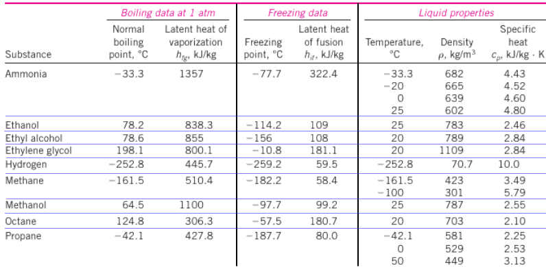
Thermal Conductivity - Reference [4] - for air: k [W/m-K] = a + b.T + c.T2 + d.T3 where T is in [K]. a = -3.933E-04 [W/m-K], b = 1.018E-04 [W/m-K2], c = -4.857E-08 [W/m-K3], d = 1.521E-11 [W/m-K4]. There is 25% increase in thermal conductivity of air in the temperature range 15 ~ 100 [°C] and hence a constant thermal conductivity may yield lower heat transfer rate. For air at 50 [°C], k = 0.02735 [W/m-K] and at 100 [°C], k = 0.03095 [W/m-K]. In STAR: Field function for temperature dependent thermal conductivity: thCondAir = 1.52e-11 * pow($Temperature,3) - 4.86e-8 * pow($Temperature,2) + 1.02e-4 * $Temperature - 3.93e-4 where T is in [K]. As per the formula, thCondAir = 0.0262 [W/m-K] at T = 300 [K]. Reference [2] - Soft Rubber: 0.13 [W/m-K], Glass Fiber: 0.043 [W/m-K], Urethane Rigid Foam: 0.026 [W/m-K]
Water: Reference [1] - Suggested curve fits for water in the range 0 ≤ T ≤ 100 [°C]: ρ (kg/m3) ≈ 1000 - 0.0178 ( T[°C] - 4[°C] )1.7 ± 0.2%. Viscosity: ln(μ/μ0) ≈ [-1.704 - 5.306.z + 7.003.z2] where z = 273 [K]/T [K] and μ0 = 0 1.788 E-3 [kg/(m.s)] ≡ [Pa.s]. Reference [2] - Thermal conductivity of Olive and Peanut Oil: 0.168 [W/m-K], Rubber Natural: 0.28 [W/m-K], Rubber-vulcanized-soft: 0.13 [W/m-K], Rubber-vulcanized-hard: 0.16 [W/m-K]
Critical point: there are multiple ways to describe critical point. "The highest temperature at which the liquid phase of a substance can exist", "The temperature above which a gas cannot be liquefied no matter how much pressure is increased", "The end-point of a phase equilibrium curve where the distinction between liquid and gas phases disappears". The critical point for water is 373.9 [°C] and pressure 22.06 [MPa] = 220.6 [bar] = 217.7 [atm]. For CO2, it is 31 [°C] and 72.8 [bar]. While dealing with systems related to power plants such as boiler, one needs to be familiar with following chart.
Use material properties as tabulated data function of p and T: In STAR-CCM+ use "Physics Simulation > Materials > Setting Material Properties Methods > Using Table (T, P)". In ANSYS FLUENT, File > Table File Manager... > Read...
Emissivities
Reference [2]: "HEAT AND MASS TRANSFER by YUNUS A. ÇENGEL from University of Nevada and AFSHIN J. GHAJAR from Oklahoma State University"
| Material | Temperature [K] | Emissivity |
| Aluminium | ||
| Polished | 300-900 | 0.04-0.06 |
| Commercial sheet | 400 | 0.09 |
| Heavily oxidized | 400-800 | 0.20-0.33 |
| Anodized | 300 | 0.8 |
| Steel | ||
| Polished sheet | 300–500 | 0.08-0.14 |
| Commercial sheet | 500-1200 | 0.20-0.32 |
| Heavily oxidized | 300 | 0.80 |
| Stainless Steel | ||
| Polished sheet | 300–1000 | 0.17-0.30 |
| Lightly oxidized | 600-1000 | 0.30-0.40 |
| Heavily oxidized | 600-1000 | 0.70-0.80 |
| Non-metals | ||
| Teflon | 300–500 | 0.85-0.92 |
| Rubber soft | 300–500 | 0.86 |
| Paints black | 300 | 0.88 |
| Wood | 300 | 0.90 |
Some other fluids widely used in industry: Engine Coolant (Ethylene Glycol + Water Mixture where mono-ethylene glycol - MEG and diethylene glycol - DEG are collectively known as EG), Transmission Oil (Nytex 810): density of 902 kg/m3 and dynamic viscosity of 5.77E-2 [Pa.s]. Following table is referenced from corecheminc.com/ethylene-glycol-water-mixture-properties. For more information, refer to product brochure published by MEGlobal, the manufacture of E.G. through a joint venture between The Dow Chemical Company and Petrochemical Industries Company of Kuwait headquartered in Dubai.
| Temperature | Ethylene Glycol Solution (% by volume): cP (centi-Poise) = 0.001 [Pa.s] | ||||||
| °C | 25 | 30 | 40 | 50 | 60 | 65 | 100 |
| -17.8 | Below F.P. | Below F.P. | 15 | 22 | 35 | 45 | 310 |
| 4.4 | 3.0 | 3.5 | 4.8 | 6.5 | 9.0 | 10.2 | 48 |
| 26.7 | 1.5 | 1.7 | 2.2 | 2.8 | 3.8 | 4.5 | 14 |
| 48.9 | 0.9 | 1.0 | 1.3 | 1.5 | 2.0 | 2.4 | 7.0 |
| 71.1 | 0.65 | 0.7 | 0.8 | 0.95 | 1.3 | 1.5 | 3.8 |
| 93.3 | 0.48 | 0.5 | 0.6 | 0.70 | 0.88 | 0.98 | 1.4 |
| 115.6 | above B.P. | above B.P. | above B.P. | above B.P. | above B.P. | above B.P. | 1.8 |
| 137.8 | above B.P. | above B.P. | above B.P. | above B.P. | above B.P. | above B.P. | 1.4 |
| Temperature | Ethylene Glycol Solution (% by volume) g/cc = 0.001 x [kg/m3] | ||||||
| °C | 25 | 30 | 40 | 50 | 60 | 65 | 100 |
| -40 | Below F.P. | Below F.P. | Below F.P. | Below F.P. | 1.12 | 1.130 | Below F.P. |
| -17.8 | Below F.P. | Below F.P. | 1.080 | 1.100 | 1.110 | 1.120 | 1.160 |
| 4.40 | 1.048 | 1.057 | 1.070 | 1.088 | 1.100 | 1.110 | 1.145 |
| 26.7 | 1.040 | 1.048 | 1.060 | 1.077 | 1.090 | 1.095 | 1.130 |
| 48.9 | 1.030 | 1.038 | 1.050 | 1.064 | 1.077 | 1.820 | 1.115 |
| 71.1 | 1.018 | 1.025 | 1.038 | 1.050 | 1.062 | 1.068 | 1.049 |
| 93.3 | 1.005 | 1.013 | 1.026 | 1.038 | 1.049 | 1.054 | 1.084 |
| 115.6 | above B.P. | above B.P. | above B.P. | above B.P. | above B.P. | above B.P. | 1.067 |
| 137.8 | above B.P. | above B.P. | above B.P. | above B.P. | above B.P. | above B.P. | 1.050 |
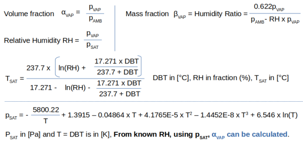
Material Properties of Moist Air: Water vapours are integral part of ambient air typically denoted as %RH (Relative Humidity). The presence of water vapour significantly changes specific heat capacity specially at high relative humidity values. The content of moisture in air is also denoted by Specific Humidity which is a ratio of the amount of water vapor in the air to the amount of dry air in a given volume. To calculate properties of the moist air, refer to this page.
As per NASA Technical Note "EQUATIONS FOR THE DETERMINATION OF HUMIDITY FROM DEWPOINT A N D PSYCHOMETRIC DATA":
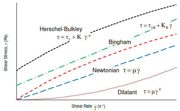
Non-Newtonian Fluids: Most of the fluids behave such that shear stress is linear function of strain rate with zero initial threshold value of shear stress. However, there are some material where shear stress is non-linear function of strain rate with non-zero initial threshold value of shear stress (yield point) before which flow cannot start. Various type of such material also known as Bingham plastic and Herschel-Bulkley are described below.
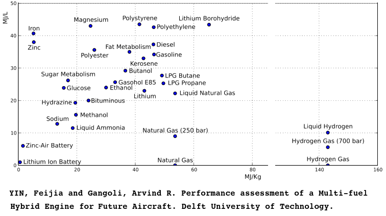
Two key attributes of a fuel is energy density which can be J/kg or J/L. From storage point of view, the value of energy per unit volume [J/L] is important. As one can see from the following table, Hydrogen ranks low in terms of energy per unit volume.
Thixotropic Materials - these are another extreme case of non-Newtonian fluids where viscosity changes when loaded by stress and the fluid becomes less viscous. Thixotropic materials display a viscosity that decreases both with shear rate and time of shear. The viscosity is termed both history- and shear-dependent (shear thinning). Examples include paints, grease, creams, jelly, gels, wax, glues and adhesives, concrete mix...
Real Gas Properties: gases do not obey ideal gas law at all temperatures and pressures. The departure from ideal gas behaviour is captured by Real Gas Properties (RGP) table. CFD Solver Modelling guide has detailed explanation of RGP table. In ANSYS FLUENT, pressure-inlet, mass flow-inlet, and pressure-outlet are the only inflow and outflow boundaries available for use with the real gas models.
To define Real Gas Properties, Power license is required. Energy model should be turned ON to access this option. Select User Defined EOS under Equation of State as shown below to define material properties say density as tabulated data of temperature and pressure.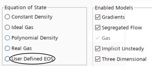
Equivalent Orthotropic Thermal Conductivity
Enter up to 10 layers. Units: thermal conductivity k in [W/m-K], thickness, length and width in [mm]. If length or width is left blank, all layers assumed to share the same lateral area. Click Calculate to compute equivalent kx, ky, and kz.
Assumptions: each layer is homogeneous and isotropic. Area (length x width) is provided for all layers. In-plane k values are computed as volume-weighted averages, through-thickness values were computed as harmonic mean — series thermal resistances. If length or width is not provided for all layers — in-plane k computed by thickness-weighted rule-of-mixtures (volume fractions by thickness). If layers have different lateral areas, provide Length and Width for each.
Training Project: the validation of 1D calculation above with 3D numerical simulation using ANSYS Fluent or OpenFOAM is a good project for trainee engineers - it will provide not only a hands-on of the CFD simulation methods but also give exposure to basics of validation of simulation results.
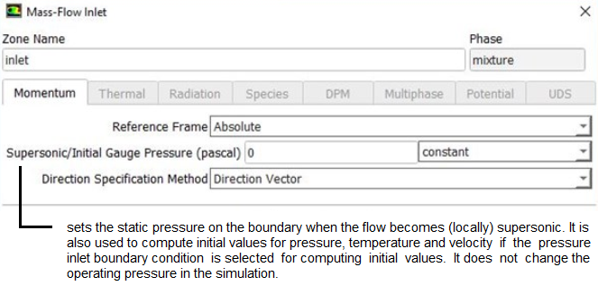
Inlet
This is the 1st member of the pair of boundary conditions which are must for any CFD calculations in a forced convection situation. Of course a natural convection case does not required any inlet or outlet. The primary consideration of an inlet B.C. is to select between the Velocity, Mass Flow Rate, Static Pressure and Total Pressure based on the actual information available about the operating conditions of the system and robustness of the solver, (the matrix inversion) algorithm which keeps running till solution is achieved. While tempting to use velocity inlet B.C. care needs to be taken to account for change in cross-sectional area when an arc is represented by a set of connected lines.
Set Mass Flow Inlet boundary conditions using TUI: /define/b-c/mass-flow-inlet zNAME y y n 0.75 n 50.0 n 10000 n y n n y 2 5
| zNAME | Name of the zone |
| y | Reference Frame: Absolute? |
| y | Mass Flow Specification Method: Mass Flow Rate? |
| n | Use Profile for Mass Flow Rate? |
| 0.75 | Mass Flow Rate in [kg/s] |
| n | Use Profile for Total Temperature? |
| 50 | Total Temperature [in unit selected i.e. K or °C] |
| n | Use profile for Supersonic / Initial Gauge Pressure? |
| 10000 | Supersonic Initial Gauge Pressure (in [Pa]) |
| n | Direction Specification Method: Direction Vector? |
| y | Direction Specification Method: Normal to Boundary? |
| n | Turbulence Specification Method: K and Epsilon? |
| n | Turbulence Specification Method: Intensity and Length Scale? |
| n | Turbulence Specification Method: Intensity and Viscosity Ratio? |
| y | Use profile for reference frame Z-component of rotation axis? |
| 2 | Turbulent Intensity [%] |
| 5 | Turbulent Viscosity Ratio |
Some other considerations during application of Inlet B.C. is "Fully Developed Flow" Vs "Developing Flow". For example, if you are a beginner learning tips and trick of CFD by trying to simulate HTC and correlating it with Dittus-Boelter equation, make sure that the flow regime is fully developed. Sometimes, the inlet of the problem set-up is moved upstream the actual location to get the flow a bit developed. Specification of turbulence parameters (turbulent kinetic energy, TKE and turbulent eddy dissipation, TED) should be based on actual measurement of as far as possible. When there are any source of momentum such as centrifugal fan in the computation domain or sharp edges, the overall result gets affected by the turbulence set at the inlet. Followings are the methods to specify turbulence:
- Specify TKE [m2/s2] and TED [m2/s3] explicitly
- Turbulent Intensity [%] and Turbulent Viscosity Ratio (TVR) [-]
- Hydraulic Diameter [m] and Turbulent Intensity [%]
- Turbulent Intensity [%] and Length Scale [m]
- External Flows
- Length Scale = 0.07 x L
- Turbulent Intensity: Based on upstream condition
- Turbulent Viscosity Ratio: 1 < TVR < 10
- Internal Flows
- ~ Length Scale = Hydraulic Diam.
- Turbulent Intensity: 0.16 x Re-1/8
- Turbulent Viscosity Ratio: 1 < TVR < 10
Recirculation Inlet: in many cases there is an internal source of momentum (such as fan) which circulates the air inside a closed domain or a source of momentum as well as heat sink such as a chiller unit. Such flow systems do not have an inlet or outlet in the sense defined earlier. Such source of momentum can be modeled as fan boundary condition if its performance characteristics is known. However, in case a fixed flow boundary type has to be applied, ANSYS FLUENT has option to use Recirculation Inlet activated using TUI (rpsetvar 'icepak? #t) (models-changed) whereas Siemens STAR-CCM+ has option to use Interface of type "Fully Developed Flow". This is a direct way of implementing recirculation conditions though Expressions and UDF can also be used to implement this condition. In recent versions say V2020 onwards, the provision of Named Expressions have eliminated the need of some of the basic UDFs.
Sometimes the information for mass flow rate is provided in [mmscfd] which stands for million-standardcubic-feet/day where one 'm' is used for thousand and two 'm' are use for million. The important feature is the term 'standard' which refers to the method of converting actual value into standard conditions (1 atm and 0 °C). Thus, in CFD simulation involving high pressure and temperature, the density should be used at those operating conditions but mass flow rate should be estimated by calculating gas density at standard conditions.
DPM and inlet boundary conditions: For particle injection, most of the time it is easier to specify particles of uniform diameter unless detail information about particle size distribution is known. There is a method Rosin-Rammler equation based on assumption that "an exponential relationship exists between the droplet diameter 'd' and the mass fraction of particles or droplets with diameter > d". This is a curve-fit and hence ≥ 3 set of information is required for combination [diameter, mass fraction of particles of diameters > d]. The curve-fit shall result in four parameters which need to be specified: minimum diameter, maximum diameter, mean diameter (size parameter) and spread parameter (the exponent in Rosin-Rammler equation).
Profile Boundary Conditions
In STAR, a parabolic inlet velocity in radial coordinate system can be specified as: v(r) = V0 × (1 - (r2/R2)) --- ${V0} * (1 - (pow(${RadialCoordinate}, 2) / pow(${Radius}, 2))). The profile in Cartesian coordinate system can be expressed as: 1.5*(pow($$Centroid[2], 4)) + 2.5 * (pow ($$Centroid[2], 3)) - 0.75 *(pow($$Centroid[2], 2)) + 10.0 where $$Centroid[0] refers to X-coordinate, $$Centroid[1] refers to y-coordinate and $$Centroid[2] refers to z-coordinate. Note arrays in STAR are 0-indexed inline with convention followed in JAVA programming language.Outlet
A outflow boundary condition in Ansys Fluent will impose zero gradient for all the flow variables.
Boundary source: Inlet can also have a boundary source define to model heat sources such as solar radiation.
When radiation is active, the emissivity at each inlet and outlet boundary can be defined while specifying boundary conditions in the associated inlet or outlet boundary dialogue box. An appropriate value for Internal Emissivity has to be entered. ANSYS FLUENT includes an option to take into account the influence of the temperature of the gas and the walls beyond the inlet and outlet boundaries, and specify different temperatures for radiation and convection at inlets and outlets. This is useful when the temperature outside the inlet or outlet differs considerably from the temperature in the enclosure. In the flow inlet or outlet dialogue box, select Specified External Temperature in the External Black Body Temperature Method drop-down list, and then enter the value of the radiation boundary temperature as the Black Body Temperature.
It is highly likely you may observe temperatures in your model that are lower than expected. Ensure that the external radiant conditions give good account of the surroundings. Alternatively, you can turn off radiative heat loss through inlets and outlets by specifying "Internal Emissivity" = 0 which otherwise may be effectively radiating to a temperature of 0 [K].
Wall Boundary - What is physical and mathematical significance?
Walls are required to store a liquid or contain the expansion (mixing) of gases. Since all the fluid flow has to be contained inside walls or at least in a channel, wall B.C. is natural extension into the numerical simulation process. Wall are not only the source of 'turbulence' that gets generated in the flow domain, its surface characteristics becomes important if certain assumptions gets violated.
In any CFD software it is not necessary to create 'named' 2D regions for the walls. This is because any faces of a 3D region which do not explicitly have a 2D region assigned to them, are automatically assigned to the default B.C. 'wall' having 'Adiabatic' condition. In case one wishes to create walls such as "Isothermal / Rotating / Heat Flux Wall", it must be created during the pre-processing.
Typically, there is no flow across the wall boundary conditions. However, in case of permeable or porous walls, flow does occur across the wall. Similarly, in case of suction or blowing (for example transpiration cooling in Gas Turbine Blades), the mass flow rate specifications are required on the wall boundary conditions.
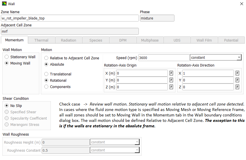
In a stationary domain with rotating wall is valid only if wall motion is entirely tangential. If there is any normal component, rotating wall shall push the adjacent fluid element. Hence, it must be modelled as rotating fluid with stationary walls relative to rotating domain.
The setting for wall boundary conditions in ANSYS FLUENT is shown below: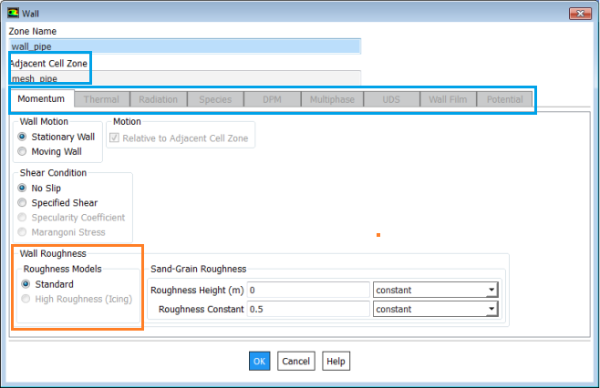
- No-slip: Velocity of fluid at wall boundary is same as fluid velocity.
- Free slip: Velocity component parallel to wall has finite value (computed by the solver), but the velocity normal to the wall and shear stress both set to zero. Zero gradients for other field variables are not enforced in slip wall conditions.
- Wall Roughness: Walls are assumed to be hydraulically smooth so long the "sand roughness height" is inside the Laminar Sub-layer. Roughness is also called "Rugocity". Typically roughness is caused by small protrusions over the mean surface of a manufactured component. Any such "technical roughness" can be converted into a "equivalent sand roughness".
- ks = Sand Roughness Height [m] or [μm], k+ = ks/h where h is characteristic height of viscous sub-layer. Please refer to the turbulence modelling page for definition of viscous sub-layer.
- ks >> h: In this case roughness element take up all of the boundary layer and hence the viscosity is of no further importance (also call "Fully Rough Regime" where flow is independent of Reynolds Number.
- ks < h: Here roughness elements are still completely within the purely viscous sub-layer and the flow can be assumed to be "hydraulically smooth", that is, there is no difference as compared to the ideal smooth surface.
- Roughness Reynolds number, Reks is defined as Reks = ρ.u+.ks/μ and the surface roughness condition can be defined as:
- Reks ≤ 5: hydraulically smooth and the wall surface roughness need not be activated in CFD simulations
- 5 < Reks ≤ 70: transitionally smooth and wall surface roughness can be activated in CFD simulations though the impact of pressure drop or wall shear stress may not always be noticeable
- Reks > 70: fully rough regime and wall surface roughness need to be activated in CFD simulations.
- Contact Resistance: By default, the walls are assumed to have zero thickness. This setting can be used specify the typical contact resistance between fluid-solid such as fouling factors or the contact resistance between solid-solid. If the thickness of the wall needs to be modelled to account for conductive resistance normal to the plane only (no conduction along the plane), contact resistance value can be specified as [t/k] where t = thickness of the wall and k is thermal conductivity of the solid.
Some typical value of thermal conductance when air gaps are not evaluated are tabulated below (reference: "A Textbook oo Heat Transfer" by Lienhard IV and Lienhard V) -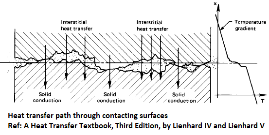 Thus, for a ceramic - aluminium pair (such as in electronic chips) with contact surface area of 20 [mm] x 20 [mm], the thermal contact resistance would be in the range 1.67 ~ 0.30 [K/W]. Note that contact resistance is also a function of contact area, higher the surface area lesser thee contact resistance in [K/W]. For a ceramic - ceramic pair having contact surface area of 10 [mm] x 10 [mm], the thermal contact resistance would be in the range 20.0 ~ 3.33 [K/W].
Surface Pair Thermal Conductance [W/m2K] Copper - Copper 10,000 ~ 25,000 Aluminium - Aluminium 2,200 ~ 12,000 Ceramic - Metals 1,500 ~ 8,500 Stainless steel - Stainless steel 2,000 ~ 3,7000 Ceramic - Ceramic 500 ~ 3,000 - Baffles or Zero Thickness Wall or Two-sided Wall: A wall that forms interface between regions such as fluid-solid interface are called two-sided walls. When a wall is used to represent thin baffle, a fluid zone will be on each side of the wall. Such zones in FLUENT are automatically split into two identical wall Jones by adding suffix '-shadow'. They are coupled unless "Temperature or Heat Flux" boundary conditions are used on one of them. In other words, different temperature and heat flux values can be specified on the two sides of a Zero Thickness Wall.
- Shell Conduction: If a thickness is specified to a wall then thermal resistance across the wall thickness is imposed though conduction is considered in the wall in the normal direction only. If the walls are of nearly uniform thickness and the conductive heat transfer needs to be accounted for both in-plane and through-the-plane conduction, this feature can be used. The user needs to specify only the thickness and thermal conductivity of the solid as described in case of contact resistance.
Shell conduction can be used to account for thermal mass in transient thermal analysis problems such as thermal soaking (ramp-up) or thermal cool-down. It can also be used for multiple junctions and allows heat conduction through the junctions. Shell conduction can be applied on boundary walls as well as internal walls. Fluxes at the ends of a shell conducting wall are not included in heat balance reports. These fluxes are accounted for correctly in the ANSYS FLUENT solution, but are not listed in the flux report.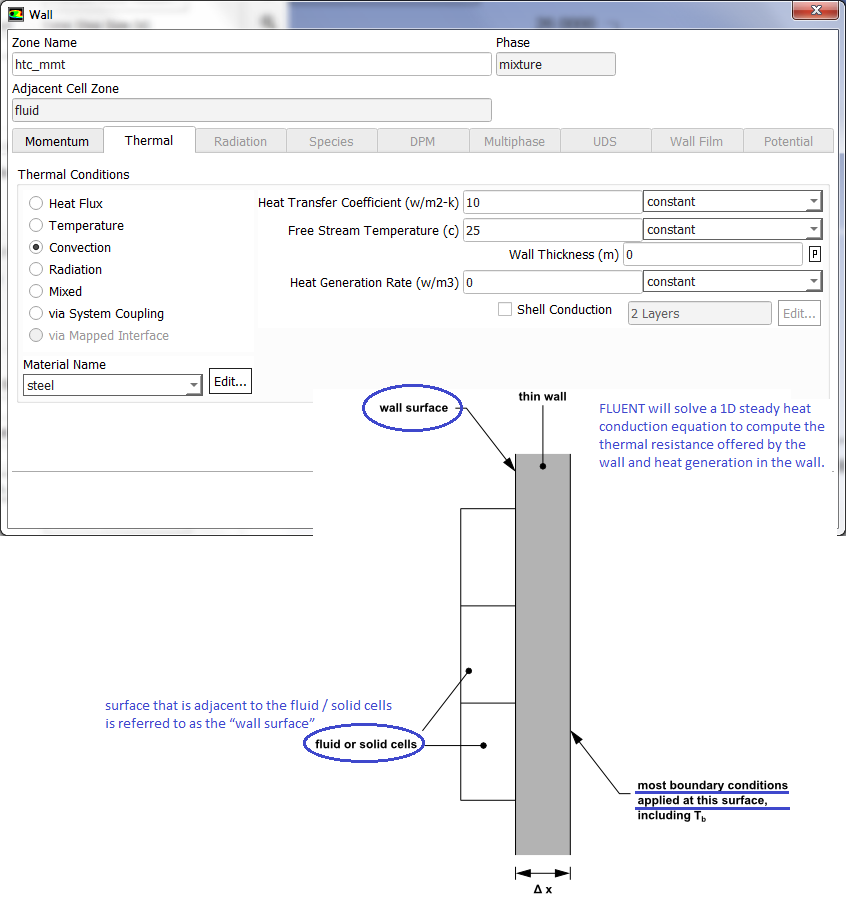
FLUENT creates a shadow wall by adding suffix ':external' to the walls on which shell conduction is switched ON. Shell conduction model uses virtual nodes or virtual cells and hence there are no real physical locations of these cells. Arbitrarily large thickness for the shell conduction model can be specified. The sides of the shell zone need boundary conditions as well. The sides will be adiabatic if they are connected to face zones having a boundary condition type other than a 'wall'. If the attached wall has shell conduction, the common sides at the junction will be coupled.
- TUI to delete all shell conduction zones: mesh modify-zones delete-all-shells. Note that once shell conduction settings are turned off (deleted), the old data file (solution with shell conduction) cannot be read with new case file (without shell conduction).
- Wall Motion:
Radiation: Walls can be defined as opaque, semi-transparent or transparent to model radiation effects. An opaque wall participate by absorbing, reflecting and emitting radiation. A semi-transparent wall will transmit radiation through it as well. On the other hand, these properties of a solid may be different for infra-red radiation and solar radiation. For example, glass is transparent to solar radiation (that is solar radiation can pass through a glass wall without any reflection/absorption) whereas it is opaque/semi-transparent to infra-red radiation (it traps these waves by refection and absorption).
- For S2S model in FLUENT, a "partial enclosure" (i.e. view factor calculations disabled for walls, inlet and exit boundaries that are not participating in the radiative heat transfer) can be defined by turning off the Participates in S2S Radiation option in the Radiation tab of the Wall dialogue box for each relevant wall. /define/b-c/set wall wall_x () radiation-s2s-surface? yes q
- Similarly, view factor calculations for any inlet or exit boundary can be disabled.
- In ANSYS FLUENT, a wall boundary cannot be turned on to participate in view factor calculations unless it is part of a fluid wall.
- The semi-transparent boundary condition can be appropriate, for example, when modelling for glass panes in air. Note that for semi-transparent walls, the internal emissivity defined under thermal conditions is ignored. Emissivity and absorptivity on a semi-transparent surface can only be effected volumetrically in the wall thickness as a consequence of the wall material absorption coefficient.
- External Wall Temperature T∞ and External Emissivity εEXT: q" = heat flux to the wall = HTC x (TW - TF) + q"RAD = εEXT . σ (T∞4 - TW4) where q"RAD is Radiant heat flux to the wall from within the domain, TW is wall surface temperature and TEXT is the temperature of the radiation sink or source on the exterior of the domain.
For Surface to Surface (S2S) radiation, a new geometrical entity type named 'patch' in STAR-CCM+ and "Surface Clusters" in ANSYS FLUENT is used. They refer to either the individual boundary cell (tri, quad or poly) or a group of these boundary cells. In FLUENT, for view factor calculations mesh (fluid zone) needs to be present between the participating surfaces. The solver clubs these many number of elements on a surface and stores their weighted average value of view factors as the cluster view factor for radiation heat transfer calculations. The default settings in STAR-CCM+ for radiation patches are 100, meaning that the patch/face proportion is 1:1 and each face translates into 1 radiation 'patch'. Setting the value say 25, each radiation 'patch' shall cover 100/25 = 4 boundary faces. The automatic option in ANSYS FLUENT requires (default 10) a value for "Maximum Faces per Cluster" under the "View Factor and Clustering" window. Though view factor calculation is a computationally expensive process, it is only needed to be performed once as the mesh and the computational domain remains the same during the simulation.
TUI for Radiation Setting: /define/models/radiation discrete-ordinate? , , , , where comma is used to accept default or values defined earlier. The 4 inputs needed are (1)Number of θ divisions (2)Number of φ division (3)Number of θ pixels and (4)Number of φ pixels.
The TUI to define emissivities for the walls is: /define/b-c/wall <wall zone name> , , , , , , , , , 0.40 , , , , where the emissivity is 0.40. This TUI command sets the wall as OPAQUE. Also note that the TUI operation does not accept multiple wall zones or wildcard characters such as wall_rad_* to accept all wall zones starting with wall_rad.
However, recent versions (certainly V22 onwards), has a way to directly change specific boundary value. The emissivity of walls can be set as /define/b-c/set wall w_1 w_2 w_3 () in-emiss no 0.80 q where no is answer to question "Use Profile for Internal Emissivity?". For all walls of type shadow: /define/b-c/set wall (*shadow) in-emiss no 0.75 q
The sequence of input and questions are: Wall-Zone-Name, Wall-Thickness, Use-Profile-for-Heat-Generation-Rate? Heat-Generation-Rate, Material-Name[...]: Change Current Value?, Use-Profile-for-[...]?, [...] (Constant or Expression), Enable Shell Conduction?, Use Profile for Internal Emissivity?, Internal Emissivity (Constant or Expression), Radiation BC Type [Opaque]: Change Current Value?, Diffusion fraction (constant or expression) [1], Use Profile for Convective Augmentation Factor?, Convective Augmentation Factor (Constant or Expression)[1].
A wall and *-shadow pair have two adjacent zones (fluids or fluid-solid), one to each of the wall and *-shadow pair. For that reason, roughness and internal emissivities have to be set correctly. In ANSYS FLUENT, for conjugate heat transfer cases, FLUENT creates a clone of the actual wall with suffix 'shadow' added to the original name of the wall. To define roughness and emissivity, in the boundary condition panel - ensure that the wall selected has a solid zone defined as "Adjacent Cell Zone" which can be either the original wall or the cloned wall.
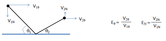
DPM (Discrete Particle modelling): In DPM simulations dealings with solid-liquid or solid-gas where particles or droplets interact with walls, the boundary conditions need to be specified as per expected behaviour. When a solid particle hits the wall, it may either reflect or get captures (stick to the wall). Elastic impact is not realistic even at particles with diameters at micron level. Hence, an appropriate coefficient of restitution need to be specified. Usually, particles travelling at lower velocity (how much lower - it is not a unique value) and smaller ones tend to get captured by the wall. The wall-particle interaction phenomena results in deposition of dust particles on solar panels, leaves of the trees, window panes and the blades of a rotating ceiling fan. Gravity can also have significant effect on dust deposition for particles with diameters > 50 [μm]. For liquid droplets, there are 4 different types of wall-droplet interactions: Splash, Stick, Rebound and Breakup. The rebound with known coefficient of restitution in normal direction (EN) and tangential direction (Eθ) is explained in following diagram.
TUI Commands for S2S Radiation
- define/models/radiation/s2s-parameters compute-clusters-and-vf-accelerated wall-vf.s2s.gz
- define/models/radiation/s2s-parameters compute-fpsc-values: Compute only fpsc values based on current settings
- define/models/radiation/s2s-parameters compute-vf-only: Compute/write view factors only
- define/models/radiation/s2s-parameters compute-write-vf "surface_vf.s2s": Compute/write surface clusters and view factors for S2S radiation model
- define/models/radiation/s2s-parameters partial-enclosure-temperature: Set temperature for the partial enclosure
- define/models/radiation/s2s-parameters print-thread-clusters: Print the following for all boundary threads: thread-id, number of faces, faces per surface cluster, and the number of surface clusters
- define/models/radiation/s2s-parameters print-zonewise-radiation: Print the zonewise incoming radiation, view factors, and average temperature
- define/models/radiation/s2s-parameters read-vf-file: Read S2S file
- define/models/radiation/s2s-parameters set-global-faces-per-surface-cluster: Set global value of faces per surface cluster for all boundary zones
- define/models/radiation/s2s-parameters set-vf-parameters: Set the parameters needed for the view factor calculations. To set number of faces per surface cluster: "define models radiation s2s-parameters set-vf-parameters , 10 , , , , , , q q" where , is to accept default values.
- define/models/radiation/s2s-parameters/split-angle: Set split angle for the clustering algorithm.
- /define/b-c/set wall wall_x () radiation-s2s-surface? yes q
View Factor Parameters:
Resolution specifies the resolution of the hemicube. The default value is set to 10. Increase the value to reduce aliasing effects that can lead to overestimated or underestimated view factors, available for Ray Tracing method only. Subdivisions specifies the number of subfaces into which each face is divided. The default value is set to 10. This parameter is only available for the hemicube method. Normalized Separation Distance specifies the ratio of the minimum face separation to the effective diameter of the face.
ANSYS FLUENT: While the hemicube method projects radiating surfaces onto a hemicube, the ray tracing method instead traces rays through the centers of every hemicube face to determine which surfaces are visible through that face. Also, the ray tracing method is OpenMP parallelized and will therefore use all available processors when performing the ray tracing calculations. As a result, the calculation time is reduced for large, complex geometries that have obstructions between the radiating surfaces (such as automotive under-hood simulations). Note that the ray tracing method does not subdivide the faces (as can be done when using the hemicube method by setting the Subdivisions or Normalized Separation Distance parameters), and so the view factors may be less accurate than those calculated using the hemicube method for surfaces that have a normalized separation distance less than 5.ANSYS FLUENT: It is recommended to use the hemicube method for large, complex models with few obstructing surfaces between the radiating surfaces, because it is faster than the adaptive method or ray tracing method for these types of models.
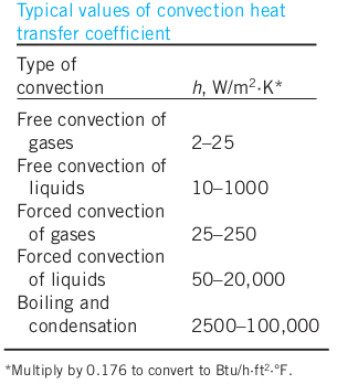
STAR-CCM+: In the view factor calculation step, deterministic ray tracing is applied to compute the factors. Rays are traced into the hemisphere above each patch using a fixed distribution of directions over this hemisphere. By default, a distribution of 1024 rays per patch is used. The number of rays per patch limits the view factor count. Therefore, with reciprocity, maximum of (2 x N) view factors per patch is generated, where N is the number of rays per patch. Thus, 1 million patches with 1024 rays/patch would produce a maximum of about 2.048 billion view factors. STAR-CCM+ provides the flexibility to use a patch resolution that is coarser than the boundary face resolution. Patches can be formed by aggregating the boundary faces from the underlying mesh. For high-resolution meshes, generally 1 patch for every 10 or so faces is used from the underlying mesh.HTC:Typical Range
Reference: "HEAT AND MASS TRANSFER by YUNUS A. ÇENGEL from University of Nevada and AFSHIN J. GHAJAR from Oklahoma State University"
Natural Convection (Buoyancy-driven Flows)
Boussinesq approximation: ρEFF = 1 - β(TWALL - TREF). Here: ρEFF= effective driving density β = coefficient of thermal expansion (equal to 1/T for ideal gas, T in [K]). Boussinesq approximation is only valid for β × (TWALL - TREF) << 1.0 say β × (TWALL - TREF) < 0.10. In other words, the temperature difference should be < 30 [K] for reference temperature of 300 [K].- Use Boussinesq approximation to start the simulation. Specify correct density and expansion factor of the fluid
- Initialize the domain with small velocity say 0.02 or 0.05 [m/s] in the direction opposite to the gravity
- Alternatively, solve a force convection flow with small velocity is expected inlet(s) and then switch on to natural convection mode
- Turn-on radiation once flow and temperature fields have stabilized
When the Boussinesq approximation is not used, in buoyancy-driven flows, the body force [Fz = (ρ - ρOP)×g] acts in the momentum equation. Here, ρOP is operating density, default method to compute the operating density in ANSYS FLUENT is by averaging over all cells.
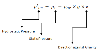
As per FLUENT User's Manual: "The boundary pressures that you input at pressure inlet and outlet boundaries are the redefined pressures as given by equation above. In general you should enter equal pressures, p'HS at the inlet and exit boundaries of your ANSYS FLUENT model if there are no externally-imposed pressure gradients. For example, if you are solving a natural-convection problem with a pressure boundary, it is important to understand that the pressure you are specifying is p'HS. Therefore, you should explicitly specify the operating density rather than use the computed average. The specified value should, however, be representative of the average value. In some cases the specification of an operating density will improve convergence behaviour, rather than the actual results. For such cases use the approximate bulk density value as the operating density and be sure that the value you choose is appropriate for the characteristic temperature in the domain."
Periodic Boundary Conditions
Strictly speaking, this is not a boundary condition. That is, any numerical simulation can proceed without it. However, this is a great tool to reduce the computational effort and resource if the flow can be envisaged to be symmetrical about a plane or pair of planes. It must be noted that there is a subtle difference between geometrical symmetry and periodicity. Periodic interfaces are treated as if one side of the interface has been translated or rotated to align with the second side of the interface. The periodic type determines the type of transformation (translational or rotational) used to map one side of the interface to the other.
- They must be in pairs.
- They have to be physically identical.
- There is a symmetry. But, unlike a symmetry BC, there is a flow normal to the BC
- The flow field in at one BC is equal to the flow field out at the other
- Types of periodic boundaries
- Translational Periodic BC: In this case the two sides of the interface must be parallel to each other such that a single translation transformation can be used to map Region List 1 to Region List 2. Flow around a single louvre in a whole array in a heat exchanger fin is an example
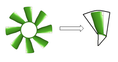
- Rotational Periodic BC: In this case the two sides of the periodic interface can be mapped by a single rotational transformation about an axis. Flow domain through an Axial Flow Fan can be reduced using rotational periodic B.C.
In solver mode: define/boundary-conditions/periodic sets boundary conditions for a zone of this type. define/boundary-conditions/modify-zones/create-periodic-interface creates a conformal or non-conformal periodic interface. define/boundary-conditions/modify-zones/make-periodic attempts to establish periodic/shadow face zone connectivity and define/boundary-conditions/modify-zones/slit-periodic slits periodic zone into two symmetry zones. define/periodic-conditions/massflow-rate-specification? enables or disables specification of mass flow rate at the periodic boundary. define/periodic-conditions/pressure-gradient-specification? Enables or disables specification of pressure gradient at the periodic boundary.
Symmetry Boundary Conditions
Strictly speaking, this also is not a boundary condition. That is, any numerical simulation can proceed without it. However, this is a great tool to reduce the computational effort and resource if the flow can be envisaged to be symmetrical about a plane or pair of planes. It must be noted that the geometrical symmetry does not guarantee symmetry of the flow. For example, side wind condition for external aerodynamics calculation requires to run the full geometry. Similarly, cases where micro-structure of flow eddies are being captured such "Large Eddy Simulation" or "DES – Detached Eddy Simulation", symmetry cannot be used owing to inherent 3D nature of the eddies.
Most of the pre-processors do not have mirror option to duplicate or copy a mesh around symmetry plane. However, note that mirror operation is also a scale (reflection) operation around the mirror plane. f(x) = -x3 is the reflection of the f(x) = x3 about the x-axis. Similarly, f(-x) reflects f(x) over the y-axis. In other words, reflection in the x axis maps y to -y, while reflection in the y axis maps x to -x. Reflection in the x axis transforms the vector (x,y) to (x, -y). In FLUENT Mesher, the scale operation on cell zones can be used to get full geometry from a symmetry half geometry.
Reflection matrices: about XY, YZ and ZX planes respectively. If the value 1 or -1 in rows 1 to 3 and columns 1 to 3 are changed to any other value, it becomes an scaling operation.| 1 0 0 0| |-1 0 0 0| | 1 0 0 0| | 0 1 0 0| | 0 1 0 0| | 0 -1 0 0| | 0 0 -1 0| | 0 0 1 0| | 0 0 1 0| | 0 0 0 1| | 0 0 0 1| | 0 0 0 1|
- By definition, a symmetry BC refers to planar boundary surface. If 2 surfaces which meet at a sharp angle & both are symmetric planes, set each surface to be a separate named boundary condition, rather than combine them into a single one.
- Velocity component normal to the Symmetry Plane Boundary = 0. Scalar variable gradients normal to the plane is also =0
- If a particle reaches symmetry plane, it is reflected back.
- Symmetric geometry doesn't necessarily imply that the flow field is also symmetric. For example, a jet entering at the centre of a symmetrical duct will tend to flow along one side above a certain Reynolds number. This is known as the Coanda effect. If a symmetry plane is this situation, an incorrect flow field will be obtained.
Volumetric Heat Sources
The heat generation in solids such as MOSFET, Capacitors, Current Carrying conductors can be modeled as volumetric heat sources [W/m3] calculated as ratio of "Total Heat Generation Rate" [W] / "Volume of the Solid" [m3]. STAR-CCM+ accepts 'Total' heat generation rate as input (specified directly to the volume) whereas in ANSYS FLUENT as on V2023 R2, the heat source needs to be applied as volumetric value. Sometimes a spreadsheet calculation needs to be performed to find out volumetric heat sources when number of volumes are too many. However, the process can be simplified using named expressions as explained in following section such as hs_mosfet = 5.0 [W] / Volume(['mosfet']).
The volumetric heat source for a current carrying conductor can be calculated as q''' = q/V = i2R / V = i2ρ*L/A/V= i2ρ*L*A/A2/V = i2ρ/A2 where i = current, ρ = eletrical resistivity, L = length and A = cross-section area. Note that volumetric heat density is independent of wire length for constant cross-section area. In case the cross-section area changes, the wire should be split to approximate it to segments of constant areas.
Sometimes volumetric heat sources can be simplified as surface heat flux though it is recommended to use this with appropriate wall thickness with shell conduction. When surface heat flux is used with zero wall thickness, the uniform value of heat flux may lead to incorrect temperature when the variation of heat transfer coefficient is high. The use to shell conduction option helps conduct the heat within the solid as it would have occurred when 3D volume zone were modelled.
The transient cooling of solids can be simplified to a steady state problem with 'virtual' heat generation rate. The formula to convert thermal inertia is: q''' = M x Cp x ΔT / tCOOL_DOWN where M is mass of the solid/liquid, Cp is the specified heat capacity and ΔT is the assumed/expected drop in temperature over a period tCOOL_DOWN. For warm-up simulation, the heat source can be specified as negative value. Note that the 3D thermal simulation using this approach may yield temperature of solid higher than assumed/expected ΔT above. This is an indication that the cooling mechanism is not sufficient either due to "lesser convection" or "lower temperature difference" between the cooling medium and the solid being cooled. And hence required drop in temperature of the solid is not possible in assumed tCOOL_DOWN. A good sanity check would be to estimate required heat transfer coefficient (HTC) value as per formula: h = [q''' x VSOLID/ASOLID] / (TMEAN - TCOOLING-FLUID) where VSOLID = volume of the solid, ASOLID = wetted surface area, TMEAN is mean temperature of the solid = (T0 - ΔT/2), T0 is the initial temperature of the solid.
Many times, material properties and volumetric heat source are function of pressure and temperature. They might be available in tabular format and a curve fit may not be possible to get a good fit. A user code in STAR-CCM+ is available at "community.sw.siemens.com/.../User-Coding-for-2-dimensional-T-p-Table-interpolation-Linux-OS" which can be adapted for ANSYS FLUENT as well. This example assumed data in the following format (say Format-1):T p q''' T_01 p_01 q_11 T_02 p_01 q_12 ... T_n p_01 q_1n T_01 p_02 q_21 T_02 p_02 q_22 ... T_n p_02 q_2n ... ...A more compact form would be as shown below (say Format-2).
T     p1      p2      p3     ...  pn
T_1   rho_11  rho_12  rho_13 ...  rho_1n
T_2   rho_21  rho_22  rho_23 ...  rho_2n
...
...
T_m   rho_m1  rho_m2  rho_m3 ...  rho_mn
Alternate to Format-2 can be shown below (say Format-3).
p     T1      T2      T3     ...  Tn
p_1   rho_11  rho_12  rho_13 ...  rho_1n
p_2   rho_21  rho_22  rho_23 ...  rho_2n
...
...
p_m   rho_m1  rho_m2  rho_m3 ...  rho_mn
Click the tabs below to get Python code which converts data in multiple (> 3) columns into 3-columns array.
def transformMultiToThreeColumns(multi_col_data):
  '''
  Transforms multi-column data into a 3-column format, the value in column
  one gets repeated for each value of data in row one. The first column shall
  contain the unique values from the original first column, he second column
  shall contain the values from the header row, excluding the first element,
  and the third column contains the corresponding values from the data rows.
  Args:
    data: A list of lists representing the input data.
  Returns:
    A list of lists representing the transformed data.
  '''
  data_3_column = []
  if not multi_col_data or len(multi_col_data) < 2:
    return data_3_column

  header = multi_col_data[0][1:]
  for row in multi_col_data[1:]:
    first_col_val = row[0]
    for i, val in enumerate(row[1:]):
      data_3_column.append([first_col_val, header[i], val])
return data_3_columnmulti_col_data = [ ["T", 1.00, 1.50, 2.00, 2.50], [300, 1.11, 1.15, 1.22, 1.25], [350, 1.05, 1.11, 1.16, 1.18], [400, 0.98, 1.02, 1.13, 1.17], [450, 0.95, 1.01, 1.04, 1.14], [500, 0.92, 0.99, 1.03, 1.13], ]
data_3_column = transformMultiToThreeColumns(multi_col_data)
for row in data_3_column: print(row)
[300, 1.0, 1.11]
[300, 1.5, 1.15]
[300, 2.0, 1.22]
[300, 2.5, 1.25]
[350, 1.0, 1.05]
[350, 1.5, 1.11]
[350, 2.0, 1.16]
[350, 2.5, 1.18]
[400, 1.0, 0.98]
[400, 1.5, 1.02]
[400, 2.0, 1.13]
[400, 2.5, 1.17]
[450, 1.0, 0.95]
[450, 1.5, 1.01]
[450, 2.0, 1.04]
[450, 2.5, 1.14]
[500, 1.0, 0.92]
[500, 1.5, 0.99]
[500, 2.0, 1.03]
[500, 2.5, 1.13]
Note that these Python codes are only to manipulate the data in required format. Both STAR-CCM+ and ANSYS FLUENT need user functions written in C and hence one shall need to write the code in C to read the arrays from CSV/TXT files and make interpolation. The simplest form of a C-code to read data from text file into [n x 3] array is described below.
#include <stdio.h>
int main() {
  FILE *fptr = fopen("data.txt", "r");
  int n_rows = 1000; int n_cols = 3; int i = 0;
  float data_2d[n_rows][n_cols];
  float Tp; float Pr; float Den;

  // Read data of file in order T, P, Density
  while (fscanf(fptr, "%f %f %f", &Tp, &Pr, &Den) == 3) {
    data_2d[i][0] = Tp; data_2d[i][1] = Pr; data_2d[i][2] = Den;
    i = i + 1
  }
  fclose(fptr);
  return 0;
}
Use while (fscanf(fptr, "%f, %f, %f", &Tp, &Pr, &Den) == 3) to read CSV file. Comma in "%f, %f, %f" mean read the comma in input and discard it.
Click the tabs below to get Python code which converts 3-columns array in multiple (> 3) columns.def threeColumnToMulti(three_col_data, first_col_header="T"):
'''
Transforms 3-column data into a multi-column format
Args: three_col_data = list of lists representing the 3-column data
Output: list of lists representing the multi-column data
'''
if not three_col_data:
print("No input array provided! Empty list returned.\n")
return []
unique_col_1 = sorted(list(set([row[0] for row in three_col_data])))
unique_col_2 = sorted(list(set([row[1] for row in three_col_data])))
multi_col_data = [[first_col_header] + unique_col_2]
for first_col_val in unique_col_1:
new_row = [first_col_val]
for second_col_val in unique_col_2:
value = ""
for row in three_col_data:
if row[0] == first_col_val and row[1] == second_col_val:
value = row[2]
break
new_row.append(value)
multi_col_data.append(new_row)
return multi_col_data
three_col_data = [
[300, 1.0, 1.11],
[300, 1.5, 1.15],
[300, 2.0, 1.22],
[300, 2.5, 1.25],
[350, 1.0, 1.05],
[350, 1.5, 1.11],
[350, 2.0, 1.16],
[350, 2.5, 1.18],
[400, 1.0, 0.98],
[400, 1.5, 1.02],
[400, 2.0, 1.13],
[400, 2.5, 1.17],
[450, 1.0, 0.95],
[450, 1.5, 1.01],
[450, 2.0, 1.04],
[450, 2.5, 1.14],
[500, 1.0, 0.92],
[500, 1.5, 0.99],
[500, 2.0, 1.03],
[500, 2.5, 1.13] ]
multi_col_data = threeColumnToMulti(three_col_data, "T")
for row in multi_col_data:  print(row)
['T', 1.00, 1.50, 2.00, 2.50]
[300, 1.11, 1.15, 1.22, 1.25]
[350, 1.05, 1.11, 1.16, 1.18]
[400, 0.98, 1.02, 1.13, 1.17]
[450, 0.95, 1.01, 1.04, 1.14]
[500, 0.92, 0.99, 1.03, 1.13]
import numpy as np
def bilinear_interpolation(grid, x_var, y_var, x, y):
  '''
  Args:
    grid (np.array): A 2D array representing the data (dependent variable)
    x_var (np.array): 1D array of x - independent variable 1
    y_var (np.array): 1D array of y - independent variable 2
    x (float): The value of x to interpolate at
    y (float): The value of y to interpolate at
  Returns: The interpolated value at (x, y).
  '''
  # Find the grid indices surrounding the point
  x_idx = np.searchsorted(x_var, x, side="right") - 1
  y_idx = np.searchsorted(y_var, y, side="right") - 1

  #Check if interpolation points falls inside data grid
  if x_idx<0 or y_idx<0 or x_idx >= len(x_var)-1 or y_idx >= len(y_var)-1:
    return np.nan

  x1, x2 = x_var[x_idx], x_var[x_idx + 1]
  y1, y2 = y_var[y_idx], y_var[y_idx + 1]

  # Get the values of the four corners
  q11 = grid[y_idx,     x_idx]
  q12 = grid[y_idx,     x_idx + 1]
  q21 = grid[y_idx + 1, x_idx]
  q22 = grid[y_idx + 1, x_idx + 1]

  # Check for division by 0, perform the interpolation
  if x2 == x1 or y2 == y1:
    return q11
  x_weight = (x - x1) / (x2 - x1)
  y_weight = (y - y1) / (y2 - y1)

  interpolated_value = (
    q11 * (1 - x_weight) * (1 - y_weight) +
    q12 *      x_weight  * (1 - y_weight) +
    q21 * (1 - x_weight) * y_weight       +
    q22 *      x_weight  * y_weight
  )
  return interpolated_value

grid = np.array([[1, 2, 4], [4, 5, 10], [7, 8, 12]])
x_c = np.array([0, 5, 9])
y_c = np.array([0, 2, 4])
x_interp = 2.5
y_interp = 1.0
interp_value = bilinear_interpolation(grid, x_c, y_c, x_interp, y_interp)
print(f"Interpolated value at ({x_interp}, {y_interp}): {interp_value}")
import numpy as np
data = np.loadtxt('T-p-Rho.txt', skiprows=1, dtype=float)
T, P, rho = data[:, 0], data[:, 1], data[:, 2]
# T, p, rho = np.loadtxt('T-p-Rho.txt', usecols=(0, 1, 2), unpack=True)
degree = 2
A = []
# Create fit basis polynomials
# f(T, p)= c00 + c10.T + c20.T^2 + c01.p + c11.T.p + c02.p^2
for i in range(len(T)):
A.append([])
for pd in range(degree+1):
for td in range(degree+1-pd):
A[i].append((T[i]**td)*(P[i]**pd))
#(pd td) = (0 0), (0 1), (0 2), (1 0), (1 1), (2 0)
c, residues, rank, s = np.linalg.lstsq(A, rho, rcond=-1)
j = 0
for td in range(0, degree+1):
for pd in range(0, degree+1-td):
if td > 0 and pd > 0:
print(" + (%.3e)T^%d.p^%d" % (c[j], td, pd))
elif td == 0 and pd !=0:
print(" + (%.3e)P^%d" % (c[j], pd))
elif td != 0 and pd ==0:
print(" + (%.3e)T^%d" % (c[j], td))
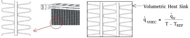
j = j + 1Volumetric Heat Exchange Coefficient: for domains such as fins in compact heat exchangers (shown below), it is not practical to model heat transfer through thin-corrugated-brazed sheets to tubes. The porous media approach used to model pressure drop in such zones can be extended to model heat source and sink as function of velocity components and local temperature.
Named Expressions
The newer versions of program FLUENT and STAR-CCM+ have option to use named expression and field functions for customized boundary conditions. These expressions can be used to define conditional cell zone source terms, models and solver settings which eliminate need to write UDF (User Defined Functions). Name of the Expressions are Case Sensitive. For example, following expression can be used to define inlet mass flow rate (kg/s) as function of static pressure (Pa) at outlet where mass flow rate is a parabolic function of pressure mdot [kg/s] = C0 [kg/s] + C1 [m.s] × pr + C2 [m^2 s^3 kg^-1] × pr2. Here pr = MassFlowAve(StaticPressure, ['Outlet']).
/define/named-expressions add exprName definition "1.25 [m/s]" q: the last entry 'q' is needed to bring the TUI to root position.
In case of field values: /define/named-expressions add exprName definition "MassFlowAve(StaticPressure, ['outlet-1', 'outlet-1']" q - here 'outlet-1' and 'outlet-2' are names of the zone of type outlet.
The boundary conditions can be defined in terms of named expressions: define/b-c/set velocity-inlet inlet () vmag "namedExpr" q where "namedExpr" is the name of the Named Expression with double quotes. vmag is a built-in variable which tells that velocity magnitude is being set or updated. As summarized in the sample journal file above: a zone type can be changed by "define b-c zone-type zName mass-flow-inlet" where zName is the name of the zone. Only the new type of zone (Mass Flow Inlet here) is needed irrespective of the original type of that zone. Once a boundary is set as type m-f-i, use following lines to make additional changes: "define b-c set m-f-i zName () direction-spec n y q" where 'n' is response to "Direction Specification Method: Direction Vector?" and 'y' is response to "Direction Specification Method: Normal to Boundary?".
"Fluent Expression Language" is an interpreted and declarative language based on Python. In ANSYS FLUENT, variables are categorized into 4 types:- Positional variables (like time)
- Field (spatial) variables (like temperature and pressure)
- Solution variables (like time-step and iteration number)
- Reduction operations (like minimum, maximum, average and sum)
In FLUENT UI, a mathematical expression can be directly used to specify boundary condition values: for example velocity at inlet can be specified as "25 [m/s]/0.0125 [m^2]". Some examples of named expressions are: arX = (Area['inlet1', 'inlet2']), solidVol = (Volume('heatSink']), Tout = MassFlowAve(StaticTemperature, ['outlet']), den = Average(Density, ['inlet_1']): Average = Area-weighted Average, Vin = 1.5 [kg/s] / den / Area(['inlet_2']), heatSrc = 5.0 [W] / Volume(['mosfet']), meanT = VolumeAve(['fluid']), r_in = sqrt(x^2 + y^2), u_in = 10.0 [m s^-1] * (1 - (r_in / 0.025 [m])**2)^(1.0/7.0)
- Units can be provided in different but consistent unit systems. For example: 5 [in/s] + 0.2 [m/s] is a valid definition of expression.
- Components of vectors can be access with .x or .y or .z suffix such as Position.x and Velocity.y, magnitude can be accessed with .mag suffix such as Velocity.mag
- There are some built-in aliases such as x (for Position.x), y, z, u for (Velocity.x), v, w, t for Time, dt for DeltaTime, iter for Global Iteration Count, T for StaticTemperature, P for StaticPressure, mf for MassFraction, mass for CellVolume*Density
- Variable names are typically combined words after capitalizing first letter of each word such Density, Velocity, StaticPressure, StaticTemperature, DynamicViscosity, EffectiveViscosity, ThermalConductivity, TurbulentViscosity, TurbulentKineticEnergy, TurbulentViscosityRatio, TurbulentDissipationRate, AreaAve
- Valid units are: mm, cm, m, km, in, ft, yd, mile, s, min, hr, day, mg, g, kg, ton, lb, rad, deg, K, C, F, R, rev min^-1, ml, litre, gallon, Pa, psi, mm Hg, in water, torr, atm
Heat Transfer Rate
The heat transfer rate has unit of [W/m2] or [cal/cm2]. However, there is a similar unit [kWhr] - this is measure of energy and 1 [kWhr] = 1,000 [W] x 3,600 [s] = 3,600,000 [J] = 3.6 [MJ]. kWhr is usually used to denote electrical power consumption while dealing with large values. In many cases such as solar radiation the energy flux is represented as [kWhr/m2/day] which will translate into average value of 1000 [W] × 3600 [s] / [24×3600] = 41.67 [W/m2]. The use of kWhr is mainly because the users are charged for energy consumption and not the rate of energy [power] consumption. Thus, a device which consumes 2 [kW] and runs for 15 hours a day will consume 30 [kWhr] = 108 [MJ].
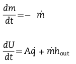
Filling and Emptying Process
"Heat Transfer Characteristics for Practical Hydrogen Pressure Vessels Being Filled at High Pressure" by Peter L. WOODFIELD et. al. Filling and emptying processes are mass accumulation and depletion process - they are not fluid flow problems in strict sense. The process is inherently transient as the mass of the simulation domain change with time. The equation to be solved are: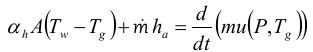
Hypersonic Flows
"Simulation of Hypersonic Flow Fields Using STAR-CCM+" by Peter G. Cross and Michael R. West: Aero-mechanics and Thermal Analysis Branch, Weapons Airframe Division. Excerpts: "Hypersonic flight (i.e., flight in excess of Mach 5) produces high temperatures that activate certain physical processes, including temperature-dependent properties, thermodynamic nonequilibrium, dissociation, and ionization, normally dormant for slower flight regimes. When simulating hypersonic flow, it is very important to model these additional physical processes, which require the inclusion of specialized models into the flow solver. However, the resultant simulations are much more challenging to solve than typical lower speed flow problems. As a result, the common practices used for simulating lower speed flows are often unsuitable when applied to the higher speed problem."Heat Exchanger modelling
Except shell and tube heat exchangers, for most engineering problems it is impractical and sometimes impossible to correctly model individual fins and tubes of a heat exchanger core. In cross-flow heat exchangers such as automotive radiators, air is called primary fluid (the heat sink) and water or coolant as auxiliary (secondary) fluid (the heat source). There are multiple approaches to model such heat exchangers when combined with surrounding systems and sub-systems.
The heat exchanger models were designed for 'compact' heat exchangers, implying that the primary fluid side flow is unidirectional. The auxiliary fluid is assumed to flow through a large number of parallel tubes, which can optionally double back in a serpentine pattern to create a number of passes. One can independently choose the direction of principal auxiliary fluid flow, the pass-to-pass direction and the direction of external primary fluid flow. Pressure loss is modeled as a momentum sink in the momentum equation and heat transfer is modeled as a heat source in the energy equation. One of the simplest option it to model volumetric heat source as function of frontal velocity: q''' = a.v + b.v2 where if q''' is [W], a and b have units [kg.m/s2] and [kg/s] respectively. If q''' has unit of [W/m3], a and b should have units [kg/m2/s2] and [kg/m3/s] respectively.
| Lumped Model | Macro Model | Dual Cell Model | |
| Accounts for the pressure loss and auxiliary fluid heat rejection | Simple-effectiveness-model | Number-of-Transfer-Units (NTU) model | Number-of-Transfer-Units (NTU) model |
| Core modeled as volumetric heat source | Compute auxiliary fluid inlet temperature for a fixed heat rejection or total heat rejection for a fixed auxiliary fluid inlet temperature | NTU method for heat transfer calculations | |
| - | Auxiliary flow is modeled as 1D flow | Auxiliary flow modelled on a separate mesh (other than the primary fluid mesh) | |
Heat Exchangers Models in STAR-CCM+
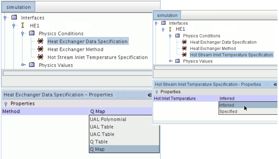
Heat Exchangers models are used to replicate the transfer of heat between two fluid streams - hot fluid and cold fluid. Applications include air conditioner evaporators, condensers, charge air coolers, radiators, electric heaters, and electronic devices. There are two options available:- Single stream option: in this case only one of the fluid streams (usually the cold stream) is modeled explicitly - by specifying the heat exchanger enthalpy source, while the second stream is assumed to have a uniform temperature that user specifies. This is activated by using option Heat Exchanger for Energy Source Option for the individual Region node.
- Heat Exchanger Exit Temperature Specification is used to choose between specifying the heat transfer rate and predicting the outlet temperature or vice versa.
- When this condition is chosen to be 'Inferred', the heat transfer rate can be specified by accessing the Heat Exchanger Energy Transfer physics value node.
- For a heater, the hot stream [e.g. coolant path in automotive radiator] is assumed to have an infinite thermal capacitance and the specified heat exchanger temperature TH refers to the constant temperature of the hot stream.
- For specified heat exchanger energy transfer rate Q, the inlet cold stream [e.g. air in automotive radiators] temperature TCI, and the cold stream specific heat CpC, an energy balance could be used to predict the cold stream exit temperature TCO as TCO = TCI + Q / CpC / mC where mC is mass flow rate of the cold fluid.
- Heat Exchanger First Iteration: This node specifies the iteration from which the heat exchanger enthalpy source is active and begins its contribution to the source term of the energy equation.
- It is recommended to active the source term when the flow is beginning to conform to its expected pattern, at least in terms of direction. As per user manual, 50 iterations is a good estimate to get a reasonable conformity.
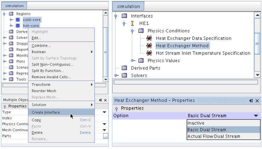
- Dual stream option: here both the streams are modeled explicitly by defining two overlapping regions and creating a heat exchanger interface between them. This model supports
- fluid-solid interface where the heat exchange occurs between a solid region and a fluid region and
- fluid-fluid interface where the heat exchange takes place between two fluid regions. For a fluid-fluid type heat exchanger, following options are available for specifying heat transfer rate in the heat exchanger:
- UAL Polynomial [UAL is function of cold flow velocity], UAL Table [UAL is a table of the cold flow velocity], UAL Map [map of curves to specify the UAL directly when multiple heat exchanger curves]: UA refers to the product of the Overall heat transfer coefficient (U) and the Area of the heat exchanger (A). UAL refers to the local (or cell value of) heat transfer coefficient (in W/K), with L referring to local.
- UAG [U.A Global] Table
- Q Table [table of the cold stream mass flow rate for one value of hot stream mass flow rate], Q Map [series of curves from which it calculates UAL].
- Basic option: This option solves for a simpler version of the energy equation using only the convective term and the source term to yield a solution. Heat Exchanger Topology:
- When using the basic option, ensure that the core mesh is constructed of uniform cells.
- In other words, all the cells in the heat exchanger region must be of comparable cell volume, as the cell volumes do not enter the calculation of the UAL table in the basic model.
- The accuracy of results that the actual dual stream heat exchanger predicts does not depend on the uniformity of the mesh.
- The topology must contain two identical regions with a different continuum associated with each region.
- Both the regions [hot and cold streams] should be created from the same mesh continuum. To ensure this, copy the [core region of the radiator] region after the volume mesh has been generated.
- Once the two overlapping regions exist, the heat exchanger interface can then be created by selecting the two regions and choosing Create Interface from the right-click menu. While selecting the two regions, select the region representing the cold stream before the region representing the hot stream.
- The mesh alignment option should be activated so that a conformal match is obtained across mesh interfaces. STAR-CCM+ does not automatically generate a conformal mesh across interfaces for the trimmed cell mesh type. Operations > Automated Mesh > Meshers > Trimmed Cell Mesher node and activate Perform Mesh Alignment.
- Create a block shape part around the core which required for the volumetric controls that define mesh refinement. Geometry > Parts node and select New Shape Part > Block.
- Actual option: UAL Map method is available with the actual dual stream heat exchanger option only.
- In both the options, heat is added or removed from the core cells as a source or sink term in the corresponding fluid energy equation. It is assumed in this section that both the streams exist only in a single phase (liquid or gas) and no phase change occurs inside the heat exchangers.
CFX Recommendation on pair - combination of boundary conditions
| Solver Behaviour | Inlet | Outlet |
| Most Robust | Velocity or Mass Flow Rate | Static Pressure |
| Somewhat Robust | Total Pressure | Velocity or Mass Flow Rate |
| Sensitive of Guess (Initialization) | Total Pressure | Static Pressure |
| Unreliable | Static Pressure | Static Pressure |
| Not possible (divergence guaranteed) | Any | Total Pressure |
FLUENT Recommendation on pair - combination of boundary conditions
| Solver Behaviour | Inlet | Outlet |
| Most Robust | Velocity or Mass Flow Rate | Static Pressure |
| Somewhat Robust | Velocity or Mass Flow Rate | Outflow or Outlet-vent |
| Only for incompressible flows | Velocity Inlet | Outflow |
| Not available | Any | Mass Flow Rate |
| Not for compressible | Specified Velocity | Any |
FAN Boundary Conditions
A fan is considered to be infinitely thin, and the discontinuous pressure rise across it is specified as a function of the velocity through the fan. The relationship may be a constant, a polynomial - of the form a + b*x2 + ... , or piecewise-linear, or piecewise-polynomial function, or a user-defined function. In FLUENT, a zero thickness plane can be used to represent a fan. However, in CFX a volume is required to represent fan as momentum source coefficient. The general momentum source in CFX has unit of [kg/m3-s2]. The source can be linearized for better convergence and stability which has unit of [kg/m3-s].
- Fan should be modelled so that a pressure rise occurs for forward flow through the fan.
- Since the fan is considered to be infinitely thin, it must be modeled as the interface between cells, rather than a cell zone. Thus the fan zone is a type of internal face zone (where the faces are line segments in 2D or triangles/quadrilaterals in 3D).
- Thus, when mesh is read into ANSYS FLUENT, the fan zone is identified as an interior zone. Interior types boundaries don't have a strict 'boundary' or 'interface' conditions, they simply pass information along. Values at interior faces follow the interpolation and reconstruction rules. Coupled walls are similar in that they mostly pass information along but they have interface conditions (they match fluxes).
- You can use the Surface Integrals dialogue box to report the pressure rise through the fan as described by following steps.
- Create a surface on each side of the fan zone - just upstream and downstream to create two new surfaces.
- In the Surface Integrals dialogue box, report the average Static Pressure just upstream and just downstream of the fan. The pressure rise through the fan is difference of downstream and upstream values.
- While generating contour plots, turn off the display of node values to see the different values on each side of the fan. If node values are displayed, the cell values on either side of the fan will be averaged to obtain a node value, and you will not see distinct (pressure, temperature, velocity ...) values on the two sides of the fan.
Fan Swirl Conditions: The fans and rotating devices can be modeled either in detail using MRF and SMM approach or using pressure jump boundary conditions. While using simplified approach where fan P-Q curve (head developed vs. flow rate) is used, one important factor is to model the swirl or tangential components. Most of the manufacturer provides only flow rate and head developed. Hence, only the axial velocity can be deduced using flow rate and annulus area. CFD simulation and design engineers have to rely on past data or those available in public domain such as conference paper and dissertations.
In ANSYS FLUENT, the values of tangential and radial velocity components can be specified on the fan surface as polynomial functions of the radial distance from the fan centre. They are typically of the form u(r) or u(θ) = Σairn for -1 ≤ n ≤ 6.[1] "INVESTIGATIONS ON THE SWIRL FLOW CAUSED BY AN AXIAL FAN: A CONTRIBUTION TO THE REVISION OF ISO 5801" by Philipp MATTERN et al and [2] Master's thesis titled "Use of experimental data to generate swirl velocity in the FLUENT Fan Model" by Ligong Yang contains good information about swirl components of axial fans. Following image is referenced from reference [1].
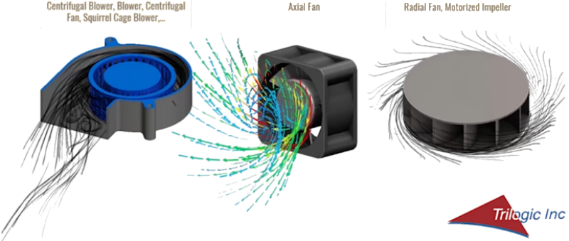
Rotating Domains
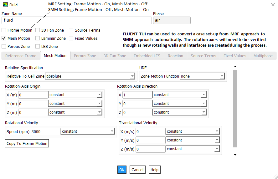
Let (x0, y0, z0) is the centre of circle passing though 3 points (x1, y1, z1), (x2, y2, z2) and (x3, y3, z3). From equality of distance (radius): (x0 - x1)2 + (y0 - y1)2 + (z0 - z1)2 = (x0 - x2)2 + (y0 - y2)2 + (z0 - z2)2. This simplifies to following set of equations. Note that this is valid only when the points are truely 3D that is the circumcircle is not aligned with either of the axes.
2(x1-x2) x0 + 2(y1-y2) y0 + 2(z1-z2) z0 = (x12 - x22) + (y12 - y22) + (z12 - z22) ... [1]2(x2-x3) x0 + 2(y2-y3) y0 + 2(z2-z3) z0 = (x22 - x32) + (y22 - y32) + (z22 - z32) ... [2]
2(x3-x1) x0 + 2(y3-y1) y0 + 2(z3-z1) z0 = (x32 - x12) + (y32 - y12) + (z32 - z12) ... [3]a1 x0 + b1 y0 + c1 z0 = d1 ... [4]
a2 x0 + b2 y0 + c2 z0 = d2 ... [5]
a3 x0 + b3 y0 + c3 z0 = d3 ... [6]
Note that the solution of this set of equations is trivial as there are infinite number of points which can be at equal distance from the three given points. The centre we are looking for is the point which is co-planar with the 3 given points. This requires some special mathematical treatment to find the coordinates of that unique point.For 2D plane when it is aligned to one of the Cartesian planes (XY or YZ or ZX):
| First point | X11: | X12: | ||
| Second point | X21: | X22: | ||
| Third point | X31: | X32: | ||
In the image above, the red lines should be defined as hub to respective zones and dotted lines as shrouds. Some programs have built-in capability to identify hub and shroud if the two keywords are present in boundary names. Hence, it is recommended to name a boundary zone as "shroud_upstream" and "hub_downstream" to get the hub and shroud identified automatically during post-processsing.
POROUS JUMP Boundary Conditions
This is opposite to the fan boundary conditions define above and like fan is also is considered to be infinitely thin membrane, and the discontinuous pressure drop across it is specified as a function of the velocity through the fan. The relationship may be a constant, a polynomial - of the form a + b*x2 + ... , or piecewise-linear, or piecewise-polynomial function, or a user-defined function. There is no similar boundary conditions available in CFX.
- It should be modelled so that a pressure drop occurs for forward flow through the porous jump.
- Porous jump should be used (instead of the full porous media model) whenever possible because it is more robust and yields better convergence.
- The porous jump model is applied to a face zone, not to a cell zone.
- By default ANSYS FLUENT uses and reports a superficial velocity inside the porous medium, based on the volumetric flow rate, to ensure continuity of the velocity vectors across the porous medium interface.
- You can use the Surface Integrals dialogue box to report the pressure drop through the POROUS JUMP membrane as described by following steps.
- Create a surface on each side of the fan zone - just upstream and downstream to create two new surfaces.
- In the Surface Integrals dialogue box, report the average Static Pressure just upstream and just downstream of the porous jump membrane. The pressure drop through the membrane is difference of upstream and downstream values.
- While generating contour plots, turn off the display of node values to see the different values on each side of the fan. If node values are displayed, the cell values on either side of the fan will be averaged to obtain a node value, and you will not see distinct (pressure, temperature, velocity ...) values on the two sides of the fan.
Porous Domains
Flow geometry such as heat exchangers with closely spaced fins, honeycomb flow passages in a catalytic converters, screens or perforated plates used as protection cover at the from of a tractor engine ... are too complicated to model as it is. They are simplified with equivalent performance characteristic, knowns as Δp-Q curve. These curves are either generated using empirical correlations from textbooks or using a CFD simulation for small, periodic / symmetric flow arrangement. The simplified computational domain is known as "porous zone" in case it is represented as a 3D volume or pressure or porous jump in case it is represented as a plane of zero thickness. In a similar fashion, the performance data of a fan can be specified including the swirl component.Examples of porous materials: note that a material which does not allow convection of fluid (e.g. brick, soil, cotton...) may allow diffusion of the fluid (brick, cotton...) such as water. In general, most of the applications of porous domain in CFD simulations refer to convection phenomena such as flow through the radiator core and honeycomb in a catalytic converter.
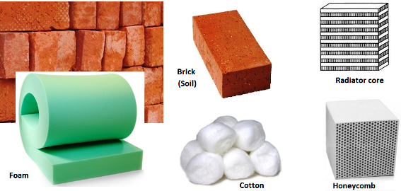
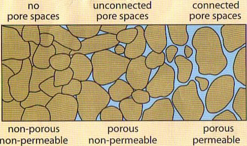
All the porous media formulation take the form: Δp = -L × (A.v + B.v2) where v is the 'superficial' flow velocity and negative sign refers to the fact that pressure decreases along the flow direction. The 'superficial velocity' is calculated assuming there is no blockage of the flow. L is the thickness of the porous domain in the direction of the flow. Here, A and B are coefficients of viscous and inertial resistances.
Porosity (γ) provides information on the overall pore volume of a porous material and is defined as the ratio of the non-solid volume (voids) to the total volume of the porous domain. The air permeability and porosity are inter-dependent, an increase in porosity (the free space) should lead to decrease in permeability (resistance to the air flow). vSUPERFICIAL = γ vREAL where vREAL is the actual velocity that can be observed or measured in the pores of the porous media. Since the measurements of velocity in such micro-channels are difficult, a superficial velocity is used which is computed the mean velocity with respect to some reference area. The image below describes a simple arrangement of porous domain in a duct.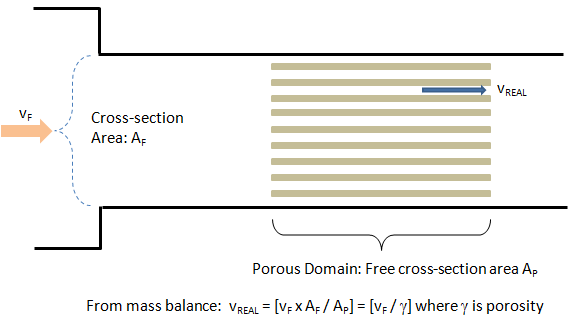
In FLUENT and CFX, the equation used is: Δp/L = -(μ/α.v + C2.ρ/2.v2) where α is known as 'permeability' and μ is the dynamic viscosity of fluid flowing through the porous domain. Note that FLUENT takes 1/α as input for porous regions. This is a measure of flow resistance and the unit of permeability (α) is [m2]. Other unit of measurement is the darcy [1 darcy = 0.987 μm2], named after the French scientist who discovered the phenomenon. The unit of inertial loss coefficient (C2) is [m-1]. A good knowledge of soil permeability, also termed hydraulic conductivity is needed for estimating the quantity of seepage under dams and dewatering to facilitate underground construction. The degree of pore saturation with water is one of significant factors affecting the soil water permeability. The permeability coefficient has unit of [m/s] and is calculated by Q.L/A/H where Q is the leakage flow rate [m3/s], L is the length of height of porous domain [m], A is cross-section area [m2] and H is applied hydraulic head [m]. The value of soils varies from 10-4 to 10-10 [m/s]. Clay is the most porous sediment but is the least permeable which acts as an aquitard, impeding the flow of water.
Inertial loss coefficient is known as Quadratic Loss Coefficient in CFX. An alternate formulation in CFX is in terms of Linear Loss Coefficient [kg/m3/s] and Quadratic Loss Coefficients [kg/m4] which are defined as A and B respectively above or Pv and Pi below.
STAR-CCM+ uses the expression Δp/L = -(Pv.v + Pi.v2) for a porous domain. Here Pv is Viscous Loss Coefficient and has unit [kg/m3/s] and Pi is known as Inertial Loss Coefficient having unit [kg/m4]. Note that it is the coefficient of v2 which is called Inertial which is contrary to the fact that viscous pressure drop is proportional to v2.
The pressure drop is usually specified as Δp = ζ/2·ρ·v2 where ζ is 'equivalent loss coefficient' and is dimensionless. Darcy expressed the pressure gradient in the porous media as v = -[K/μ]·dP/dL where 'K' is the permeability and 'v' is the superficial velocity or the apparent velocity determined by dividing the flow rate by the cross-sectional area across which fluid is flowing. All the programs FLUENT, CFX and STAR-CCM+ uses superficial velocity.Steps to find out viscous and inertial resistances:
- Calculate the pressure drop vs. flow velocity data [Δp-v] from empirical correlations or wind-tunnel test or simplified CFD simulations.
- Divide the pressure drop value with thickness of the porous domain. Let's name it as [Δp' vs. v curve].
- Calculate the quadratic polynomial curve fit coefficients [A, B] from the curve Δp' vs. -v. Ensure that the intercept to the y-axis is zero.
- In STAR-CCM+ these coefficients 'A' and 'B' can be directly used as Pv and Pi which are viscous and inertial resistance coefficients respectively.
- Divide 'A' by dynamics viscosity of the fluid to get inverse of permeability that is 1/α to be used in ANSYS FLUENT as "viscous resistance coefficient".
- Divide 'B' by [0.5ρ] where ρ is the density of fluid, to get C2 to be used in ANSYS FLUENT as "inertial resistance coefficient".
- The method needs to be repeated for the other 3 directions. If the flow is primarily one-directional, the resistances in other two directions need to be set to a very high value, typically 3 order of magnitude higher.
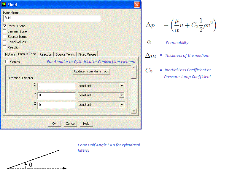
Darcy Law for Porous Media
This is the basic law governing the flow of fluids through porous media such as soil, rocks and sand beds. This is analogous to other linear phenomenological transport laws namely Ohm’s law for electrical conduction, Fick’s law for solute diffusion and Fourier’s law for heat conduction. Note that Darcy’s law is a macroscopic law will hold true over regions that are much larger than the size of a single pore.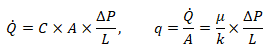
- Q = Volumetric flow rate [m3/s]
- A = cross section area of the flow passage [m2
- L = Length of flow path along the direction of flow [m]
- ΔP = pressure drop along the direction of flow = [p - ρgh] [Pa], ρ = density of fluid [kg/m3], g = acceleration due to gravity [m2/s], h = height along the direction of gravity [m]
- C = constant of proportionality [m2/Pa.s] = μ/k, μ = dynamic viscosity of fluid [Pa.s], k = permeability [m2]
Dupuit-Thiem equation (based on Darcy Law in cylindrical coordinate system) is a widely used formula to estimate pressure drop across the wall for a known (oil extraction) flow rate in a circular reservoir that has a constant pressure at its outer boundary.
Unit Vector between 2 Points: In case porous domain is not aligned to any coordinate direction, the direction of unit vector along the flow and across the flow directions can be estimated from following JavaScript program. Note that empty field is considered as 0.0. There is no check if a text value is specified in the input fields and the calculator will result in an error.
| First point - X1: | |
| First point - Y1: | |
| First point - Z1: | |
| Second point - X2: | |
| Second point - Y2: | |
| Second point - Z2: | |
Porous Loss Coefficient Calculator
Note that the loss coefficients are assumed to be (and most of the time they are so) parabolic. Hence, only 3 sets of points are required to derive the parabolic equation. It is recommended that the first point is close to no-flow conditions, second point close to the mid-point of operation and the last point towards the highest flow rate conditions. In the table below, Pi refers to pressure drop across the porous domain at Vi. Air is assumed to be the working fluid. Sutherland law is used to find out viscosity of air at specified temperature.
| Thickness of HX | TH | [mm] | |
| First point | V1 | [m/s] | |
| First point | P1 | [Pa] | |
| Second point | V2 | [m/s] | |
| Second point | P2 | [Pa] | |
| Third point | V3 | [m/s] | |
| Third point | P3 | [Pa] | |
| Gas Temperature | Tg | [°C] | |
| Gas Pressure | Pg | [kPa] | |
Example calculation: x = {0.0 1.0 2.5}, Y = {0 50 75}, m1 = 50.0, m2 = 16.67, A = -13.33, B = 63.33, C = 0.0. The parabola generated by the curve fit coefficients looks like as shown below. Note that a parabola with local maxima towards higher value of X-axis may have a negative value of A or B.
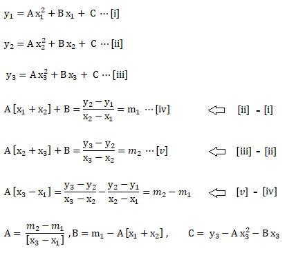
Examples of Porous Media
One of the frequent application of porous media formulation is the heat exchangers such as automotive radiators, inter-coolers, oil-cooler and honeycombs in catalytic converters. The porous formulations can also be used in Fabric Ducts used in HVAC systems. These ducts an either be "permeable only textile fabric where air is squeezed between loose fibres" or ducts with micro-perforations with laser cut holes as low as 0.2 [mm]. Micro-perforations allow creation of variety of low velocity air patterns to suit local cooling needs. In porous fabric ducts, air is allowed to pass through the fabric with the air-flow rate controlled by the fabric weave and the internal static pressure. In non-porous fabric, no air can pass through the fabric weave and air-flow is delivered through orifices and other venting options (nozzles, micro-perforations) to achieve desired air-flow.Porosity provides information on the overall pore volume of a porous material and is defined as the ratio of the non-solid volume (voids) to the total volume of the non-woven fabric. The air permeability and porosity of fabric duct are inter-dependent. An increase in porosity (the free space) should lead to decrease in permeability (resistance to the air flow). From flow point of view, a volume based definition of porosity may not provide a direct relation to the the flow velocity which depends on flow area perpendicular to the flow direction.
Dust Accumulation in Air Filters: There are many application of air filters such as automotive air cleaners. Dust Holding Capacity (DHC) is one of the key parameters of such filters. The filter are orthotropic porous media where the porous loss coefficients are different along the 3 directions. However, any CFD simulations to deal with dust accumulation will be a transient simulation where the behaviour of porous domain will change depending upon duct collection level and spatial distribution. This is because filter may not collect dust uniformly and hence permeability will change non-uniformly. For most practical applications, change in pressure drop can be assumed to be a linear function of duct loading (the amount of dust trapped in filters). How does one model the trapping of dust particles in the pores of the filter? Neither the filter pores nor the diameters of the particles are uniform in size and shape!
Convergence Troubleshooting Strategies for Porous Media
The rate of convergence slows a porous region is defined such that pressure drop is relatively large in the flow direction (e.g. the permeability is low or the inertial factor is large). This slow convergence can occur because the porous media pressure drop appears as a momentum source term yielding a loss of diagonal dominance in the matrix of equations solved. The best remedy for poor convergence of a problem involving a porous medium is to supply a good initial guess for the pressure drop across the medium. You can supply this guess by patching a value for the pressure in the fluid cells upstream and/or downstream of the medium. It is important to recall, when patching the pressure, that the pressures you input should be defined as the gauge pressures used by the solver (i.e. relative to the operating pressure defined in the simulation).
Another possible way to deal with poor convergence is to temporarily disable the porous media model and obtain an initial flow field without the effect of the porous region. Once an initial solution is obtained, or the calculation is proceeding steadily to convergence, enable the porous media model and continue the calculation with the porous region included. (This method is not recommended for porous media with high resistance.)
Simulations involving highly anisotropic porous media may, at times, pose convergence troubles. This issue can be addressed limiting the anisotropy of the porous media coefficients to two (102) or three (103) orders of magnitude. Even if the medium's resistance in one direction is infinite, it is not needed to set the resistance in that direction to be greater than 1000 times the resistance in the primary flow direction.
Tortuosity
Tortuosity - derived from work 'tortuous' - is a measure of the geometric and flow path complexity of a porous medium. A molecule often has to traverse a path that is several times longer than the straight line between its original source and destination. Tortuosity is a ratio that characterizes the tortuous and meandering (convoluted) pathways of fluid convection and/or diffusion through the media.In the fluid mechanics of porous media, tortuosity is the ratio of the length of a streamline to that of the straight-line distance between those points. A measure of deviation from a straight line. It is the ratio of the actual distance travelled between two points, including any curves encountered, divided by the straight line distance. Tortuosity is used by drillers to describe well-bore trajectory, by log analysts to describe electrical current flow through rock and by geologists to describe pore systems in rock and the meander of rivers.
A related concept is fractal which is used to describe the effective length of rivers and used even for trading in stock markets.
Atmospheric Data
Reference: Analytic Combustion by Anil W. Date (Cambridge Press).There is decrease in atmospheric pressure and temperature with altitude as compared to height above sea level. Why sea level is considered as reference datum? This is because the liquids maintain uniform level and any point anywhere in the sea is expected to be same radial distance from the centre of the Earth.
p [Pa] = 101325 * (1 - 2.25577E-05 × H)5.2559 where altitude H is in [m].
T [K] = 288.15 - 0.0065 × H. You may use the following calculator to estimate ambient pressure and temperature at higher altitudes. There is option to chose altitude in [m] or [ft]. However, the outputs are in SI units.
| Altitude, H | |
| Unit | |
Binary Diffusion Coefficients
In situations with multi-component flows (such as leakage of fuel or refrigerant) where diffusion dominates the correct specification of binary diffusion coefficient is very important. Following table specifies value at 1 [atm] and 300 [K]. Reference: Analytical Combustion by Anil W. Date.
| Pair | Dab [m2/s] | Pair | Dab [m2/s] |
| H2O - air | 24.0E-6 | C6H6 - air | 8.00E-6 |
| CO - air | 19.0E-6 | C8H18 - air | 5.00E-6 |
| CO2 - air | 14.0E-6 | C8H16 - air | 7.10E-6 |
| H2 - air | 78.0E-6 | C10H22 - air | 6.00E-6 |
| O2 - air | 19.0E-6 | O2 - H2 | 70.0E-6 |
| SO2 - air | 13.0E-6 | CO2 - N2 | 11.0E-6 |
| NH3 - air | 28.0E-6 | CO2 - H2 | 55.0E-6 |
| CH3OH - air | 14.0E-6 | C6H14 - N2 | 8.00E-6 |
| C2H5OH - air | 11.0E-6 | C8H18 - N2 | 7.00E-6 |
| CH4 - air | 16.0E-6 | C10H22 - N2 | 6.40E-6 |
Higher Heating Value (HHV) and Lower Heating Value (LCV) for some of the common fuel: "eere.energy.gov/hydrogenandfuelcells/tech_validation/pdfs/fcm01r0.pdf"
| Fuel | HHV at 25 °C and 1 atm [kJ/kg] | LHV at 25 °C and 1 atm [kJ/kg] |
| Hydrogen | 141.9 | 119.9 |
| Methane | 55.5 | 50.0 |
| Propane | 50.4 | 45.6 |
| Gasoline | 47.5 | 44.5 |
| Diesel | 44.8 | 42.5 |
| Methanol | 20.0 | 18.0 |
Multiphase Flows
Mass Fraction to Volume (or Mole) Fraction: ensure that the sum of mass fractions add to 1.0, no checks are performed in case they do not. Typically method to check the correctness of following method is to specify same value of mass fractions (0.5 or 50%) and density for both phases, the calculated volume fractions should be equal to 0.50 (50%) for both phases.
| First phase mass fraction [%] and density [kg/m3] | β1: | ρ1: | ||
| Second phase mass fraction [%] and density [kg/m3] | β2: | ρ2: | ||
| Volume fraction of the two phases | α1: | α2: | ||
Formula to convert mass fraction to volume fraction and vice versa:
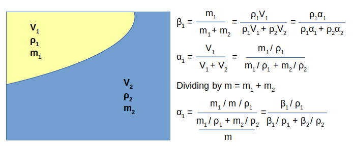
Volume Fraction to Mass Fraction: ensure that the sum of volume fractions add to 1.0, no checks are performed in case they do not.
| First phase volume fraction [%] and density [kg/m3] | α1: | ρ1: | ||
| Second phase mass fraction [%] and density [kg/m3] | α2: | ρ2: | ||
| Mass fraction of the two phases | β1: | β2: | ||
Liquid Jet Break-up
[1]:The near- and far-field break-up and atomization of a liquid jet (aerodynamic break-up of liquids) in multi-phase fluid systems fits in the broader category of multi-phase fluid flow. Secondary liquid break-up and coalescence of the droplets in the far-field atomization of the jet is also important in many application such as Diesel sprays, two-phase flow combustion and propulsion problems. The destabilization of the liquid jet close to the nozzle exit is a Kelvin–Helmholtz type of instability where surface tension acts as a stabilizing force and imposes a lower cut-off for the waves which can grow. This cut-off is given by a critical Weber number. Three forces are involved in the splitting of the liquid, namely surface tension, viscous and inertia forces.[2]: A method for aerodynamic drop break-up that has been widely implemented is known as the Taylor Analogy Break-up model or TAB. The TAB model approximates a drop as a damped oscillator system and tracks a deformation parameter. When the deformation parameter is sufficiently large, break-up is assumed.
Surface Tension and Capillary Effect
Though CFD may not be required to solve phenomena such as capillary rise, any flow geometry where surface tension effects are comparable to viscous effects should be dealt carefully. Following chart and OCTAVE (or MATLAB) scrip summarizes the effect of pipe diameter on capillary rise and volume of liquid that can be lifted.
- σ: surface tension of liquid which is measure of cohesive force between liquid molecules.
- H: Capillary rise (or depression) - lower point of the meniscus. Note that the capillary effect is the net effect of competitive forces adhesion (force between liquid and solid molecules) and cohesion. Contact angle is a constant property of liquid-solid interface and affects capillary rise.
- If contact angle is zero, the liquid surface is parallel to solid surface and the liquid is said to wet the solid completely. The equation relating to the contact angle and surface tension between all 3 interfaces namely liquid-solid, liquid-gas and solid-gas is known as Young's equation. σSL - σSG + σLG cos(θ) = 0 where S, L and G refer to solid, liquid and gas phases.
- System energy, E = σ × (2πrH) + ρ/2×(πr2H) × g
- Capillary length, LC = [2σ/ρ/g]0.5 ~ 4.0 [mm] for water at room temperature.
- Under dynamic condition when liquid level is increasing in the capillary tube, its rise is resisted by a combination of gravity, viscosity, fluid inertia and dynamic pressure.
- The timescale required to establish Poiseuille flow is, t = 4ρr2/μ where μ is the dynamic viscosity. For water and 0.50 [mm] tube: t ~ 1.2 [s], for 0.20 [mm] tube: t = 0.2 [s]. If rise timescale is less than this value, inertia of liquid mass dominates and inertial overshoot results in oscillation of liquid column about steady state (equilibrium) height.
- Note that the capillary rise predicted is 15 [m] for micro-pores (r =1.0 μm ie. 1.0E-6 m).
- The nature of wetting depends on the choice of liquid as well as on the nature of the surface. For example, water spreads on a clean glass surface but beads up on a glass sheet coated with a monolayer of dimethyloctylchlorosilane (generating a hydrophobic surface).
- Spreading of liquid also depends on the nature of the surrounding fluid. For example, oil droplets on a surface under water have a different contact angle than an oil drop in air. In both the cases, the fluid pairs are immiscible.
Surface tension and angle of contact with water and some of the non-metals are tabulated below as per www.accudynetest.com.
| Surface Tension of Water with | Abbreviation | [N/m] | [°] |
| Silicone Oxide | Glass | 0.0725 | ~ 0 |
| Poly-Vinyl-Chloride | PVC | 0.0379 | 85.6 |
| Poly-Tetra-Fluoro-Ethylene | PTFE | 0.0194 | 109 |
| Poly-Amide-6-6 | Nylon-66 | 0.0422 | 68.3 |
| Poly-Methyle-Meth-Acrylate | PMMA (Acrylic, Plexiglass) | 0.0375 | 70.9 |
| Poly-Ethylene-Terephthalate | PET | 0.0390 | 72.5 |
| Poly-Carbonate | PC | 0.0440 | 82.0 |
| Acrylonitril Butadine Styrene | ABS | 0.0385 | 80.9 |
| Poly-Ethylene | PE | 0.0316 | 96.0 |
| Poly-Propylene | PP | 0.0305 | 102 |
OCTAVE Script
Have you noticed why the water does not spill even when the water level is above the brink of a bowl!
One of the applications of capillary effect combined with fully-developed laminar (Poiseuille) flow is pipetting. Pipetting process is aspiration of a pre-determined volume of liquid by creating a vacuum above a tapered capillary tube (known as tip). The pressure in the pipette chamber during the process is in a dynamic equilibrium and is affected by the ambient pressure, viscosity, surface tension and density of the liquid, and the speed of the piston movement. The suction (aspiration) of liquid in pipette tips normally undergo following 4 phases:
- Acceleration phase: The rate of decrease of pressure the pipette chamber is higher than the rate of increase of pressure caused by reduction in gas volume due to aspirated volume of the liquid. Thus, the fluid-gas interface will tend to accelerate.
- Uniform speed phase: The pressure in the cavity reduced uniformly and is balanced by actual pressure increase due to reduction in gas volume caused by suction of fluid.
- Deceleration phase: the piston speed slows down, but the total pressure difference between the inside and outside of the pipette chamber is still high to keep the fluid moving. The liquid suction speed gradually slows down and finally maintains the balance.
- Balancing phase: the pipetting operation is completed and the static equilibrium is achieved between pressure, surface tension and hydrostatic forces.
| Regime-I | Regime-II | Regime-III | Regime-IV |
| Initial boundary effects important | Viscous effect negligible | Poiseuille flow: inertia effect negligible | Late viscous regime |
| Surface tension forces dominant | Capillary rise resisted by fluid inertia | Lucas-Washburn law applies | Fluid rise approaches steady state height |
| Capillary rise: z ∝ t2 | Capillary rise: z ∝ t | Capillary rise: z ∝ t0.5 | Capillary rise: z ∝ e-t |
Mesh and Simulation Set-up File Review
One of the challenges for any reviewer is to understand the geometry and the naming convention used for define boundary and fluid zone. Just looking at the name of the zones, no information can be gathers if it is arbitrarily designated. Some naming convention will go a long way in making the review process easier. One of the many ways is:- Use of prefixes and suffixes appropriately
- Name fluid zones as f-air- or f-water- for fluids, s-steel- for solids, por- for porous.
- Add bc-inlet-tpr for "Total Pressure" boundary condition at inlet, bc-inlet-mfl for "Mass Flow" boundary condition or bc-inlet-vel for "Velocity Inlet".
- Similarly, use bc-outlet-sprs for "Static Pressure", bc-outlet-oflo for outflow...
- Walls with specified heat flux of heat transfer coefficient should also be named appropriately such as wf-htc- or wf-hfx- or wf-tmp-
- Interfaces can start with keyword if-ff- or if-ss- or if-sf-
- Periodic boundaries can be named as prd-trn- or prd-rot-
Transient Table as Boundary Condition in FLUENT
A time-history data such as inlet temperature as function of time or mass flow rate as function of time can be specified either as an UDF (cases where analytical equations can be derived) or as a data table.The format of the standard transient profile file:
(
 (inletvel transdata 3 0)
 (time  1 2 3 )
 (invel 6 5 4 )
)
Here '3' denotes the number of data points (number of rows in tabular format). '0' indicated that data is not time-periodic, use '1' for a time-periodic dataset. 'invel' shall appear as drop-down in boundary condition panel. Note:
- All quantities, including coordinate values, must be specified in SI units.
- Profile names (e.g. 'inletvel' in this example) must have all lowercase letters
- Data can be either in column or row format.
The data set used above can also be specified as described below:
(
 (inletvel transdata 3 0)
 (time
  1
  2
  3
 )
 (invel
  6
  5
  4
 )
)
Tabular Transient Profiles
The format of the tabular transient profile file is as follows. Use TUI command "file read-transient-table fileTr.dat" to upload the data into the solver. The options "inletvel time" and "inletvel invel" shall appear in the drop-down menu of boundary condition panels.inletvel transdata 3 0 time invel 1 6 2 5 3 4
Interpolation of Results
Many a times we need to interpolate the results from previous simulations into a new simulation, such as when a new mesh is generated due to refinement or coarsening. Sometimes results may be available from simulations carried out in other software (such as FLUENT or OpenFOAM) and the field variables need to be read into a new software (STAR-CCM+). Most of the commercial program provide an options to import and export data from and into CGNS and/or CSV format. The data in this format can be used to exchange result data from one program to the other.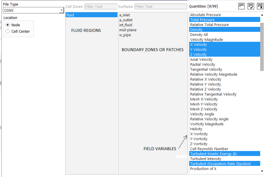
Interpolation file format: ANSYS FLUENT
2            --the interpolation file version
3            --dimension (2 or 3)
25000        --total number of points
3            --total number of fields (velocity, pressure...) included
x-velocity   --field variable to be interpolated
pressure     --field variable to be interpolated
-0.100000    --x-coordinate of first node in the list
-0.200000    --y-coordinate of first node in the list
-0.300000    --z-coordinate of first node in the list
  ...
  ...
  ...
 1.000000    --x-coordinate of last node in the list
 2.000000    --y-coordinate of last node in the list
 3.000000    --z-coordinate of last node in the list
 0.500000    --x-velocity at first node in the list
 0.100000    --x-velocity at second node in the list
 0.200000    --x-velocity at third node in the list
  ...
  ...
  ...
 5.000000    --x-velocity at last node in the list
 100.0000    --pressure at first node in the list
 200.0000    --pressure at second node in the list
 300.0000    --pressure at third node in the list
  ...
  ...
  ...
 500.0000    --pressure at last node in the list
At the end is a list of the field values at all the points in the same order as their names. The number of coordinate and field points (x-velocity and pressure in this case) should match the number given in line 3 (25000 in this case). Note that it cannot interpolate heat generation rate (W/m3), though internal energy, enthalpy, heat transfer coefficient... can be interpolated. In other words, no volumetric source/sink term can be interpolated in the fluid region. On the boundaries, all field variables are available for interpolation.
Data Export into CSV Format: ANSYS FLUENT:
The header in CSV files for FLUENT and STAR-CCM+ uses different variable names. In STAR-CCM+ variables has to be specified with appropriate units: e.g. "Absolute Pressure (Pa)", "Velocity Magnitude (m/s)", "Velocity[i] (m/s)", "Velocity[j] (m/s)", "Velocity[k] (m/s)", "X (m)", "Y (m)", "Z (m)"... Note the space between variables and unit. The x-component of velocity is accessed by Velocity[i].
Data Mapper: STAR-CCM+:
interpolateTable(@Table("VelData"), "Time", LINEAR, "VelMPS", $Time)
Here the field function type should be vector. For boundaries such as inlet, in the “Physics Values” option of the boundary in the “Method” field, select Field Function, and then right below this, select the field function defined earlier.
The name of the table is VelData, Time is the name for the first column in the .csv file, LINEAR (other option available is SPLINE) is the interpolation method creating values between the discrete time values specified in the table, VelMPS is the name of the second column in the table (corresponding to the velocity magnitude), $Time specifies that the velocity is function of time. In case velocity is function of spatial coordinates say y-axis: $${Position}[1] can be used in place of $Time to specify that the position coordinate is aligned with the y-axis (1 = y-direction, use '0' for x-direction and 2 for z-direction).
TUI in ANSYS FLUENT
Over the different versions, while new features have been added, the name of some of command have been altered and many have been removed / consolidated. For example, 'grid' has been replaced with 'mesh', /display/ set/ colors/ background white" has been replaced by "/display/ set/ colors/ graphics-theme-color white". Click here to get the list of all TUI commands available in ANSYS FLUENT.License Manager: LMTOOLS
Most of the CFD programs be it ANSYS FLUENT or STAR-CCM+ use LMTools to manage the licenses at their customers. The executable utility is installed in the same folder where main program such as ANSYS FLUENT is installed. The syntax to use LMSTAT is: lmstat [-a] [-c license_file_list] [-f [feature]] [-i [feature]] [-s[server]] [-S [vendor]] [-t timeout_value]. The purpose of each option is:- -a: Displays all information
- -c license_files: Uses the specified license files
- -f [feature]: Displays 'users' of feature. If feature is not specified, all features are displayed
- -i [feature]: Displays information from the feature definition line for the specified feature, or all features if feature is not specified
- -s [server]: Displays status of all license files listed in $VENDOR_LICENSE_FILE or $LM_LICENSE_FILE on server, or on all servers if server is not specified
- -S [vendor]: Lists all users of vendor’s features
- -t timeout_value: Sets connection timeout to timeout_value which limits the amount of time 'lmstat' spends attempting to connect to server.
Finding Names of Feature: to use -f option, one need to know the exact names of feasures. This can be found in license.dat file or check the output from -a options. lmutil.exe lmstat -s licServers -f "feature_name"
For scripting and partial automation of pre-processing, solver and post-processing activities, refer to this section of scripting page.
For dealing with file handling in Linux and Windows, refer to short summary of shell scripting.
Checklist to check adequecy of boundary conditions for steady state simulations
| No. | Checkpoint | Record [Y / N / NA] |
| 01 | Is the CAD data available in STEP format? | |
| 02 | Are the boundary condition values at inlets available: mass or volume flow rate, temperature, pressure? | |
| 03 | Are the boundary conditions at outlets available: mass flow rate, pressure? | |
| 04 | Are the boundary conditions such as surface heat sources at walls available? | |
| 05 | Are the volumetric heat generation rates available? | |
| 06 | If applicable, is the fan performance curve available? | |
| 07 | If applicable, is the pressure drop vs velocity curve available for porous domain? | |
| 08 | Are the material type and grade for all solids avaiable? | |
| 09 | Are the values of ambient conditions (temperature and pressure) available? | |
| 10 | Are the thermal conductivity values of non-standard materials available? |
References
- STAR-CCM+ User Guide Version 10.02
- ANSYS FLUENT User Guide V15.0
- Break-up and atomization of a round water jet by a high-speed annular air jet: J. C. Lasheras, E. Villermaux And E. J. Hopfinger
- modelling Aerodynamic Break-Up Of Liquid Drops In A Gas Flow With Molecular Dynamics Analogy Methods: Alexander L. Brown And Flint Pierce, Sandia National Laboratories, PO Box 5800, Albuquerque, NM, 87185-1136, USA
The content on CFDyna.com is being constantly refined and improvised with on-the-job experience, testing and training. Examples might be simplified to improve insight into the physics and basic understanding. Linked pages, articles, references and examples are constantly reviewed to reduce errors, but we cannot warrant full correctness of all content.
Copyright © 2017 - All Rights Reserved - CFDyna.com
Template by OS Templates