- CFD, Fluid Flow, FEA, Heat/Mass Transfer: Feedbacks/Queries - fb@cfdyna.com
Turbomachines
CFD Simulation approaches for Turbomachines
Multiple Reference Frame, Sliding Mesh Motion
Table of Contents: MRF Approach - Limitations | Roll, Pitch and Yaw | Flow inside a centrifugal blower for HVAC applications | Dynamic Mesh Motion | Cavitation in Pumps | Mixing Tanks or Stirred Tanks | Propellers |:| Flow and Losses in Transmission Gearboxes |*| NPSH: Net Positive Suction Head |-| Testing of Fans |=| Gas Turbines and Airfoils (*) Wind Turbines |:| WAsP - Wind Atlas Analysis and Application Program |:| Lifecycle of a Wind Farm
Geographic Information System (GIS) in Wind Energy |:| Wind Rose Diagram
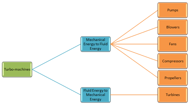
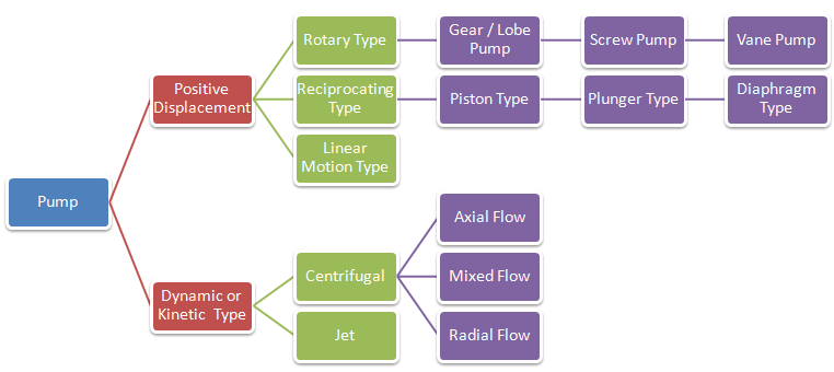
CFD simulation approach for turbomachines such as centrifugal pump and blowers, appropriateness of various modelling approaches namely Single Reference Frame (SRF), Multiple Reference Frame (MRF) or Frozen Rotor Method, Sliding Mesh Motion (SMM) along with applications to industrial problems are described in this page. Before moving to the CFD simulation aspects, following two graphics summarize the types of turbomachines available in industries. The simulation can be just one phase (liquid or gas) or multi-phase applications such as investigation into mixing effects in Gas-Liquid-Solid Stirred Reactor. The explanation on multi-phase flow simulations can be found here.
Forward-curved Blade vs. Backward-curved Blades: Two articles titled "The Difference Between Forward Curved and Backward Curved Fans" (longwellfans.com/difference-between-forward-curved-and-backward-curved-fans) and "Comparison between Forward Curved and Backward Curved Fans" (sofasco.com/blogs/article/comparison-between-forward-curved-and-backward-curved-fans) give good comparison.
Pumps need to transfer energy to the liquids and their suction (inlet) lines are at lower pressures than the discharge lines. In general, it is assumed that the inlet line is always filled with water without any traces of air or gas. However, this is not always the case. If the centreline of the pump is above the water supply reservoir and there is no check valve or the pump is started first time, there will be air present in the suction line. Centrifugal pumps with basic design features cannot remove the air from the suction line and can only start to pump the fluid after it has initially been primed with the fluid.
The term 'priming' refers to the phenomena of removing the air from the system. Types of self-priming pumps are centrifugal pumps with "separation chamber", "side channel" or "water ring pumps" and "two casing chambers and an open impeller pumps". Some self-priming pumps come with an integrated vacuum pump that ensure the pump primes at unfavourable suction pipe layouts. The self-priming feature can be imparted to a centrifugal pump by ensuring impeller is submerged in water or retains enough water when it stops. It can be achieve simply by designing a suction and discharge cavity above the centerline of the impeller or installing a check valve near the suction eye. Note that even self-priming pumps will need initial priming after commissioning.
CFD simulations of a pump is carried with known mass flow rate and known pressure at one of the boundaries. However, any simulation of a self-priming process needs to be carried out with atmospheric boundary conditions at both inlet and outlet as well as keeping the gravity on - to separate gas from liquid. Alternatively, pressure inlet and the opening at the outlet can be used as inlet and outlet boundaries in order to approximate the actual self-priming operation This makes the simulation process special and a transient simulation is necessary.
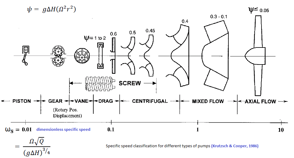
Pumps are characterized by a single value known as specific speed. There are some dimensional variants of specific speeds and some non-dimensional. Hence, utmost care should be taken to check and use appropriate units used to derive the specific speeds. ISO 5801:2017 specifies procedures for the determination of the performance of fans of all types except those designed solely for air circulation, e.g. ceiling fans and table fans. Testing of jet fans is described in ISO 13350. The aeroacoustic measurements are performed using a test rig (the so-called In-Duct method) according to the industry norm ISO 5136 where far-field noise levels are recorded inside a circular duct using three slit-tube microphones.
CFD Simulation Methods for Turbomachines
SRF: This method is used when the computational domain is axi-symmetric. This is called 'single' reference frame because only one reference frame (which is rotating) needs to be defined. This method can be used when whole geometry (the computational domain) can be assumed rotating.
Lumped Fan (FP) or Body Force Model: This method does not model the blades and hub, instead uses an interface at the location where the fan blades would be located. An experimentally obtained fan curve (pressure drop vs. flow rate) is applies as pressure rise (pressure jump or porous jump) over the interface according to the mass flow rate. The drawbacks of this model are that the velocity vectors exiting the interface of the standard LF model only have an axial component, no swirl (tangential component) and no reduced velocity where the hub would be located. These drawbacks can be reduced by adding a swirl to the outlet flow or geometrically leaving out the hub region from the interface.
MRF:This method uses more that one reference frames - at least one stationary (outer) and 1 rotating (inner). This is also known as Frozen Rotor Method (FRM) as the rotating parts are kept frozen in position and rotation is accounted for by the additional source terms through inclusion of centrifugal and Coriolis forces. Instead of the blades moving physically through the air, the air moves around the rotor blades with a corresponding angular velocity. Even for the cases where transient simulation is required, MRF method is useful for attaining initial values for time-dependent simulations because the pseudo-steady state can be reached within a few revolutions starting from zero initial velocity. MFR approach is appropriate if the flow seen from the rotating/moving frame of reference is steady along the interface. In other words, when flow is relatively uniform at the interface between the moving and stationary zones. E.g. in mixing tanks the impeller-baffle interactions are relatively weak, large-scale transient effects are not present and the MRF model can be used.
- The equations for the inner rotating region are solved in a rotating reference frame (when a rotating reference frame is used the centrifugal and Coriolis forces are included in the momentum equation). The equations for the outer stationary region are solved using a stationary reference frame. The solutions from both regions are matched at the interface between the rotating and stationary regions via velocity transformation from one frame to the other. This velocity-matching step involves the implicit assumption of a steady flow condition at the interface. The local velocity value may depend on the position of the impeller blade.
- Domain and Mesh: The accuracy of simulation result is sensitive to the selection of MRF region. It is defined so that it includes rotating parts and extends to upstream and downstream sections where a mixed-out (relatively uniform) flow field exists. MRF region can also include stationary parts if they are rotationally symmetric. The mesh (elements and nodes) inside the rotating domain including external or internal boundaries rotate as a solid body with the rotation angular speed specified about the axis of rotation.
- Walls: In order to account for wall shear, solver needs to know the speed of the wall. Any external or internal wall inside the rotating domain is assumed to rotate at the speed of the domain. If a wall defining the boundary of rotating domain is required to be defined stationary, it either needs to be specified as "counter-rotating wall" or its angular velocity needs to be defined as "0 [rad/s]". In FLUENT, this can be achieved using the feature motion "Relative to Adjacent Cell Zone" or 'Absolute'.
- Governing Equations: In both SRF and MRF methods, the momentum conservation is governed by the Navier-Stokes equations and the mass conservation is governed by the continuity equation. Both SRF and MRF methods are called steady-state approach (or pseudo-transient due to usage of pseudo time stepping) where the solution is time independent and rotation is achieved through mesh fixed in space and time. As a result, it does not model unsteady (transient) effects at the frame change interface.
- Result is influenced by 'frozen' position of rotating components (blade) with respect to the stationary parts (baffles, involute). Hence, the validity of result should be thoroughly checked when either the number of blade count is low or the speed of rotation is relatively low.
- MRF result will be inaccurate when flow crosses the interface from both directions - that is when flow enters and leaves the outer boundary of rotating domain.
- As per ANSYS user manual, the use of the realizable k-ε turbulence model with multiple reference frames is not recommended. The PRESTO! scheme for the discretization of pressure equation is recommended for solving rotary machines.
MRF Approach - Limitations:
Excerpts from "Evaluation of the Multiple Reference Frame Approach for the Modelling of an Axial Cooling Fan" by Randi Franzke, Simone Sebben, Tore Bark, EmilWilleson and Alexander Broniewicz.The fan performance curve, describing the pressure rise over volume flow rate through the fan, is commonly under-predicted when using the MRF model. This under-prediction mainly occurs at low to medium volume flow rates (radial and transitional regime), therefore it is concluded that the MRF method works best when the fan is operating in axial conditions. Liu et al. (2016) found that the thrust of a tidal current turbine was equally under-predicted with the MRF approach as the pressure rise. Furthermore, they found that the frozen rotor position has a significant influence on the flow field in the near wake. Kobayashi and Kohri (2011) showed that uniform inflow conditions are necessary in order to facilitate the transition to the moving reference frame. Apart from the operating conditions, it is also important that flow structures originating from the blades (e.g. tip vortices) are completely encompassed by the MRF domain, in order not to be split or in other ways being hindered from developing. As was pointed out by Gullberg and Löfdahl (2011) and Kobayashi et al. (2014) the performance of the MRF approach is highly dependent on the users choice of the size of the MRF. A large MRF domain has therefore been shown to give better agreement with experimentally obtained fan curves. For open fans (i.e. no ring connecting the blade tips), the radial extent is more important, due to the occurring tip vortices, while for both the open and closed fan type a sufficiently large axial extent can lead to more uniform inflow conditions and hence a better performance prediction. Therefore it can be concluded that the users choice of the MRF domain has a substantial impact on the accuracy of the results.
SMM: In Sliding Mesh Motion (rigid body motion - RBM) the rotation is achieved through moving mesh functionality which is a time dependent process and hence known as transient simulation approach. No additional source terms area added into the momentum equations. This is specially required when (a)vortices of next blade (or wake behind the blade) that have just passed upwind affect the following blades or (b)flow unsteadiness due to pressure waves which propagate both upstream and downstream.
- Note that the mesh motion can be constant speed or accelerating – the solver accommodate both situations.
- In the SMM formulation, the motion(s) of moving zone(s) is tracked relative to the stationary reference frame where the motion of any point or node in the domain is given by a time rate of change of the position vector - known as grid speed.
- SMM and DMM uses same equations where in case of DMM, has additional feature for nodes to move relative to each other. Hence, SMM can be assumed to be a subset of more general DMM method.
- Since this approach involves mesh motion it is necessary that the interface between the zones be two overlapping faces, one of which is attached to the rotating region while the other is attached to the stationary region. The interaction between the two regions is modelled by interpolating the information across these faces. No additional source terms needs to be added into the momentum equations. For each time step, nodes are rotated and the fluxes at the sliding interfaces (interface at the stationary and rotating) are recomputed.
- Time steps for transient simulation is a function of element size (Δs) at the sliding interface. The time steps should always be less that it requires a moving / rotating cells to cross past a stationary point at the interface that is Δt ≤ Δs/ω/r where ω is the rotational speed of moving domain and r is the radius of sliding interface.
- The mesh interface between rotating and stationary domains must be situated such that there is no motion normal to it.
- The common boundary or mesh interface can be any shape (including non-planar surfaces) provided the two interface boundaries are derived from a set of common geometrical entities (lines in 2D and surfaces in 3D).
- By default, the velocity of wall is zero relative to the motion of the mesh or cell zone it is attached to. For walls bounding a moving mesh this imposes the "no-slip" condition in the reference frame of the mesh. Hence, one need to modify the wall velocity boundary conditions only if it is stationary in the absolute frame and therefore moving in the relative frame. For example, shroud of a fan is a stationary wall bounding the rotating reference frame defined for the blades. Hence, its velocity should be explicitly set to ZERO.
- An interface is a MUST between rotating and stationary regions (domains or zones). Sometimes, such surface zones can be set as 'interior' instead of an interface.
- However, such 'interfaces' must be a surface of revolution having axis of revolution coinciding with the axis of revolution of the rotating zones and walls.
- The recommended practice is to chose the location of such interface(s) at the mid-way between the tip of rotating walls (or the blade tip) and the nearest stationary housing walls. Sometimes, the location of interfaces are also governed by meshing considerations (such as number of boundary layers on the walls of the blades) and free mesh size beyond this region.
- For rotating domains embedded in relative large domains (such as a fan relative very small as compared to room), the recommendation is to have the interface at a location where flow is likely to be uniform.
- Note that there is a significant difference between "Rotating Frame" and "Rotating Mesh".
DMM:
In all the cases described above, the rotating and stationary parts do not change the shape or geometry. When the parts change shape and/or size, a Dynamic Mesh Model (DMM) method is required which allow changes to be made to the mesh (as solution progresses) such as remeshing, adding and removing grid cells where necessary. 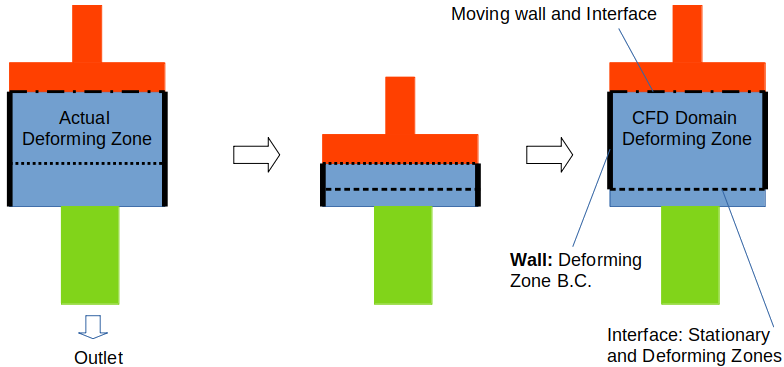
- Prescribed translation (such as motion of piston and valves in engines), rotation (motion of teeth in gear pumps) or combination of translation and rotation (motion of teeth in helical pumps). In ANSYS FLUENT, "DEFINE_CG_MOTION” is used to describe the motion of a face or cell zone. It provides solver with a velocity at every time step. ANSYS Fluent then translates this to the position of the zone given the current simulation time. DEFINE_CG_MOTION(udf_name, dt, vel, omega, time, dtime), where name defines the name of the UDF. 'dt' is a pointer to a storage that contains the dynamic mesh attributes specified by the user or calculated by FLUENT. 'vel' and 'omega' are the linear and angular velocity arrays respectively. 'time' defines the current time and 'dtime' defines the time step. These 6 variables are passed to the UDF by FLUENT, the UDF then calculates the linear and angular velocities and returns the values to ANSYS FLUENT.
- Since movement is known a priori, a sequence of meshes can be generated to accommodate the motion of the boundaries. In between those generated meshes, the mesh can be deformed (for example stretching and compression) according to the prescribed boundary movement.
- In situation where sliding interfaces need to be created in very tight clearances such as screw pumps, continuous mesh adaptation - even at every time step - might be required.
- It is when the deformation of the mesh is excessive that the deformed mesh can be replaced with a new generated one (e.g. layer addition and deletion in case of translation of boundary or linear deformation of the fluid zone).
- Note that the motion is prescribed at the solid boundaries and not at the mesh representing fluid volume which shape and size changes.
- The motion of each point and cell in the mesh needs to be calculated so that the mesh remains topologically consistent to the changes in shape and size of the fluid domain.
- During the mesh deformation process, a finite element method is used based to the Laplacian equation (∇.κ∇u = 0) for estimating the velocity and location of the mesh points, either with a constant or variable diffusivity κ. The added diffusivity controls the mesh deformation and quality.
- If the zone is a rigid body, a 'profile' or 'user-defined function (UDF)' can be used to define the motion of the rigid body or use the 6-DOF solver. The motion of a solid-body can be specified either as a profile or as a user-defined function (UDF). A profile may be defined by the following profile fields: time (time), crank angle (angle) (in-cylinder flows only), position (x, y, z), linear velocity (v_x, v_y, v_z), angular velocity (omega_x, omega_y, omega_z), orientation (theta_x, theta_y, theta_z).
- Unprescribed motion where the subsequent motion is determined based on the solution at each time step(for example, the linear and angular velocities are calculated from the force balance on a swing valve), as is done by the six degree of freedom (6DOF) solver. Motion induced by flow field which is dependent of the solution of flow field itself and found application in phenomena such as aero-elasticity and fluid-structure interactions (FSI). A noticeable difference with prescribed mesh motion case is that the deformation in this category of applications are low and as well as not known a-priori. If there is excessive deformation in solid, a high quality hexahedral mesh would be required.
- Overset mesh: this is a dynamic mesh motion option available in ANSYS FLUENT and STAR-CCM+. The Overset mesh consists always of at least two regions partially or fully overlapping each other and is useful when working with moving bodies such as swing valves. It does not require mesh modification after initialization or during the simulation. The solutions in the overlapping mesh zones are interpolated and hence cell sizes in the two meshes should be nearly same. Key concepts in overset mesh technology are: Overset Interface, Background Grid, Component Grid and Overset Boundary.
- The boundaries and interfaces are defined such that the solver divides the cells into active, inactive and acceptor groups. The inactive cells are deactivated and the flow is not solved for them while the acceptor cells are used to couple the solution between overset and background region.
- The overset region moves into the background region, and the solver automatically selects appropriate cells (active or acceptor) for the solution.
- This meshing technique can simulate a moving body with up to six degrees of freedom as well as it also permits the creation of a zero-gap interface required to simulate the full closure of valves.
- For cases such as swing valves, the closing valve disc is part of the overset region, which shall rotate according to the momentum exerted by all the forces / torques as per Newton’s second law for momentum.
- Cells in the background overlapping with valve disk becomes inactive because it is occupying that space. Later on the those cells shall get active again when disc changes its position.
Example profile for motion of the solid-body
((movement_linear 3 point)
(time  0   1   2 )
(x     2   3   4 )
(v_y   0  -5   0 ) )
((movement_angular 3 point)
(time     0   1   2 )
(omega_x  2   3   4 ) )
Typically, a DMM simulation can consist of up to 4 different zones. This is demonstrated by application of DMM for simulation of flow in an internal combustion engines. Excerpts from Theory Guide: "ANSYS Fluent expects the description of the motion to be specified on either face or cell zones. If the model contains moving and non-moving regions, you need to identify these regions by grouping them into their respective face or cell zones in the starting volume mesh that you generate. Furthermore, regions that are deforming due to motion on their adjacent regions must also be grouped into separate zones in the starting volume mesh. The boundary between the various regions need not be conformal. You can use the non-conformal or sliding interface capability in ANSYS Fluent to connect the various zones in the final model."
Standard Transient Profiles
((profile-name transient N periodic?)
(field_name-1 a1 a2 a3 .... aN)
(field_name-2 b1 b2 b3 .... bN)
.
.
(field_name-r r1 r2 r3 .... rN) )
Profile names must have all lowercase letters, time field section must be in ascending order. N is the number of entries per field. The 'periodic?' entry indicates whether profile is time-periodic or not: 1 for a time-periodic profile, or 0 if the profile is not time-periodic. An example is shown below:
((time_vel_curve transient 3 0)
(time 1  2  3)
(u   10 20 30) )
The 6DOF solver in ANSYS Fluent uses the forces and moments acting on the object in order to compute the translational and angular motion of the center of gravity of an object. The governing equation for the translational motion of the center of gravity is solved in the inertial coordinate system. Once the angular and the translational accelerations are computed from angular momentum balance and linear momentum balance respectively, the rates (angular velocity / angular displacement and translation velocity / displacement) are derived by numerical integration. The angular and translational velocities are used in the dynamic mesh calculations to update the rigid body position." For the rigid body motion of a body such as valves and diaphragms, the 6DOF solver is which computes external forces and moments on the valve by computing a numerical integration of the pressure and shear stress over the valve’s surface. It can also add additional forces or moments such as e.g. spring and mass inertia forces. When the forces and moments acting on a rigid body is estimated, it calculates the translational and rotational motion of the center of gravity of the body using equation a = 1/m . ΣF, dω/dt = 1/Inertia . Στ
Roll, Pitch and Yaw
Simulation involving dynamic mesh motion and 6-DOF requires understanding of Euler angles, roll, pitch and yawing motion. The yaw, pitch, and roll rotations can be used to place a 3D body in any orientation. A single rotation matrix can be formed by multiplying the yaw, pitch and roll rotation matrices to obtain final transformation matrix. It is important to note the order that performs the roll first, then the pitch and finally the yaw. If order is changed, transformation matrix will also change. In FLUENT, the angle of rotation or orientation about x-, y- and z-axis is denoted by φ, θ and ψ. The transformation matrix from inertial to body coordinate systems are given as: 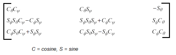
Zones and Mesh Updates in DMM
- Deforming zone: This refers to the mesh which will deform with the simulation. For example, zone or volume in 3D consisting of volume bounded by piston, liner, head and valves. The zone deforms by the valve and piston motion.
- Layering Zone: This zone represents the valve motion and it located above the valve, between valve curtain and valve stem. As the name suggest, mesh layers are added / deleted during the simulation. Whenever the mesh quality in the deforming zone or layering zone deteriorates beyond a pre-defined value, mesh is regenerated by adding or removing layers in the layering zone and remeshing the deforming zone by adding (refining) or removing (coarsening) cells (depending on if the cells are compressed or stretched during piston motion).
- Rigid Motion Zone: This is located between the layering zone and the valve. This zone keeps its geometrical shape throughout the whole engine cycle, but follows the valve motion. The function of the rigid motion zone is to capture the concave valve shape without affecting the layering zone. In this way it is easier to make new meshes at different valve lifts by simply adding or removing layers of cells in the layering zone. It also helps to preserve the mesh quality in the area of the valve exit.
- Static Zone: This zone consists of all volumes that are unaffected by boundary motion and as the name suggests they keep their geometry and shape during the whole engine cycle. This zone includes all remaining volumes in the intake and exhaust ports.
- The mesh deformation is handled in 3 ways:
- Smoothing: This is method to apply a boundary movement which retains original cells of the mesh and move the nodes to ensure certain mesh quality. This method is appropriate only when the boundaries undergo small deformation. In case of larger deformation, the layer adjacent to boundary may get so skewed that any mesh smoothing operation will not improve the quality to permissible level. The smoothing method includes three different options:
- Spring-Based Smoothing: use the edges between two mesh nodes as interconnected springs. Equilibrium state is before any boundary motion have occurred. When a displacement happen at a node, it generates a force equal to the displacement between the two nodes. Hooke’s law is used to calculate the force between the nodes. This method is used if the movement of the boundary is primarily only in one direction, resulting in no excessive stretching or compression of the cell zone
- Laplacian Smoothing: This method adjusts the mesh vertex to the center of the adjacent vertices, does not guarantee improvements on mesh quality and often lead to poor mesh quality.
- Boundary Layer Smoothing: this is often combined with another mesh motion UDF where the smoothing method is used to deform the boundary layer during the mesh motion.
- Layering: In this method, the boundary selected as a layering face has certain prescribed motion profile. All the cells adjacent to that face (in the domain marked layering) are allowed to compress and expand. All other cells of the domain perform rigid body motion - compressing or expansion as the same rate as the first layer of cells attached the layering face. This method required the layering zone to consists of either hexahedrons or prism elements. Note that this method is viable only if the moving object (boundary) is not surrounded by cells.
- Remeshing:The Remeshing method create new cells due to skewness, that is a new mesh is regenerated in the specified zone when the mesh quality deteriorates beyond a pre-defined level. An informative video on YouTube covering 6-DOF (6 Degrees-of-Freedom) solver in ANSYS FLUENT is here.
- Smoothing: This is method to apply a boundary movement which retains original cells of the mesh and move the nodes to ensure certain mesh quality. This method is appropriate only when the boundaries undergo small deformation. In case of larger deformation, the layer adjacent to boundary may get so skewed that any mesh smoothing operation will not improve the quality to permissible level. The smoothing method includes three different options:
Dynamic Mesh TUI
define/dynamic-mesh dynamic-mesh?
 Enable Dynamic Mesh? [yes] yes
 Enable In-Cylinder Option [no] no
 Enable Six DOF Solver? [no] no
 Enable Implicit Update? [no] yes
 Enable Contact Detection? [no] yes
/define/dynamic-mesh/zones create zone_x
 motion type: (stationary rigid-body deforming user-defined system-coupling)
 enter motion type: [stationary] deforming
 allow smoothing? [yes] yes
 allow local remeshing? [yes] yes
 use remeshing global values? [yes] yes
/define/dynamic-mesh/controls smoothing? [yes] yes
/define/dynamic-mesh/controls layering? [no] yes
/define/dynamic-mesh/controls remeshing? [no] yes
When using Local Remeshing method, FLUENT marks cells based on criteria set for skewness and minimum / maximum length scales. It evaluates each cell and marks the cell if it does not meet one of the following criteria:
- Skewness > the value specified by user
- Cell size < specified minimum length scale
- Cell size > specified maximum length scale
- Cell height does not meet length scale specified for adjacent boundary, e.g. a moving wall (valve or piston)
Sample UDF for 6DOF case. DEFINE_SDOF_PROPERTIES (name, properties, dt, time, dtime) specifies custom properties of moving objects for the six degrees of freedom (SDOF) solver which includes mass, moment and products of inertia, external forces and external moments. real *properties - pointer to the array that stores the SDOF properties. The properties of an object which can consist of multiple zones can change in time, if desired. External load forces and moments can either be specified as global coordinates or body coordinates. In addition, you can specify custom transformation matrices using DEFINE_SDOF_PROPERTIES. The boolean properties[SDOF_LOAD_LOCAL] can be used to determine whether the forces and moments are expressed in terms of global coordinates (FALSE) or body coordinates (TRUE). The default value for properties[SDOF_LOAD_LOCAL] is FALSE.
| #include "udf.h" | |||
| #include "math.h" | |||
| DEFINE_SDOF_PROPERTIES(valve_6dof, prop, dt, time, dtime) { | |||
| prop[SDOF_MASS] = 0.10; | /*Mass of the rigid body in [kg] */ | ||
| prop[SDOF_IZZ] = 1.5e-3; | /*Mass moment of inertia about Z axis [kg/m^2]*/ | ||
| /* Translational motion setting, use TRUE and FALSE as applicable */ | |||
| prop[SDOF_ZERO_TRANS_X] = TRUE; | /*Translation allowed in global X-Direction? */ | ||
| prop[SDOF_ZERO_TRANS_Y] = TRUE; | /*Translation allowed in global Y-Direction? */ | ||
| prop[SDOF_ZERO_TRANS_Z] = TRUE; | /*Translation allowed in global Z-Direction? */ | ||
| /* Rotational motion setting, use TRUE and FALSE as applicable*/ | |||
| prop[SDOF_ZERO_ROT_X] = TRUE; | /*Rotation allowed about global X-Axis? */ | ||
| prop[SDOF_ZERO_ROT_Y] = TRUE; | /*Rotation allowed about global Y-Axis? */ | ||
| prop[SDOF_ZERO_ROT_Z] = FALSE; | /*Rotation allowed about global Z-Axis? */ | ||
| /* Gravitational, External Forces/Moments: SDOF_LOAD_F_X, SDOF_LOAD_F_Y ... SDOF_LOAD_M_Z*/ | |||
| M = prop[SDOF_MASS]; Larm = 0.10 */ | |||
| /* DT_THETA(dt): orientation of body-fixed axis vector, DT_CG(dt): center of gravity vector, DT_VEL_CG(dt): cg velocity vector, DT_OMEGA_CG(t): angular velocity vector */ | |||
| prop[SDOF_LOAD_M_Z] = -9.81 * M * Larm * sin(DT_THETA(dt)[2] ; | |||
| Message("\n 2D: updated 6DOF properties DT_THETA_Z: %e, Mz: %e, Mass: %e \n", | |||
| DT_THETA(dt)[2], prop[SDOF_LOAD_M_Z], prop[SDOF_MASS]); | |||
| } | |||
#include "udf.h"
#define PI 3.141592654
DEFINE_TRANSIENT_PROFILE(speed, time) {
  real A = PI/12;   /*Amplitude in [rad]   */
  real f = 10.0;    /*Frequency in [rad/s] */
  real w;           /*Angular displacement */
  w = 2.0*PI*A*cos(f * time);
  return w;
}
Sign convention of rotor power in FLUENT: 'positive' value implies fluid is supplying energy to the rotor (e.g. turbine), 'negative' value implies rotor is supplying energy to the fluid (e.g. compressor or pump).
DFBI - DMM is known as DFBI in STAR-CCM+ where the DFBI (Dynamic Fluid Body Interaction) module is used to simulate the motion of a rigid body in response to pressure and shear forces the fluid exerts, and to additional user-defined forces such as weight and inertia. STAR-CCM+ calculates the resultant force and moment acting on the body due to all influences, and solves the governing equations of rigid body motion to find the new position of the rigid body. There are multiple type of DFBI features. One such feature is DFBI Superposed Rotation which superimposes an additional fixed body rotation in addition to the DFBI motion. For example, this option can be used to model rotating propellers attached to rotating and/or translating marine boats.
The 6-DOF Solver in STAR-CCM+ computes fluid forces, moments, and gravitational forces on a 6-DOF object where pressure and shear forces are integrated over the surfaces of the 6-DOF bodies. These forces and moments are used to compute the translational motion of the center of mass of the body and the angular motion of the orientation of the body. The 6-DOF body object defines the surface of the floating body for the calculations of the 6-DOF solver.
Mesh Motion in OpenFOAM: The solid body motion is defined by classes derived from common base solidBodyMotionFunction. The motion function returns a septernian which describes the motion of the body. Septernion class used to perform translations and rotations in 3D space. It is composed of a translation vector and rotation quaternion and as such has seven components hence the name 'septernion' from the Latin to be consistent with quaternion rather than 'hepternion' derived from the Greek. Quaternion are the extension of complex number system in 2D geometry to that in 3D geometry (4-dimensional division algebra discovered by Irish mathematician and physicist William Rowan Hamilton).
Immersed Solid Approach: ANSYS CFX uses an immersed solid approach to model to model steady-state or transient simulations involving rigid solid objects that can move through fluid domains such as lobe pump, gear pumps and axial flow fans. The immersed solid is represented as a moving walls (or two counter-rotating moving walls in case of gear pumps) and a source term in the fluid equations that drives the fluid velocity to match the solid velocity. Some of the limitations of this approach are: the immersed solid domain cannot undergo mesh deformation and the surfaces of the immersed solid body are not explicitly resolved by the mesh. In addition, a wall function cannot be applied to the boundary of an immersed solid and hence the accuracy of simulation results may be lower than can be obtained using mesh deformation methods or other techniques that support the use of wall boundaries to directly resolve solid surfaces.
Mixing Plane Method: MPM is available in ANSYS FLUENT. When a axial flow compressor or turbine stage needs to simulated with different values of periodic angles of rotor and stator, this approach becomes necessary. A "mixing plane" is defined at the interface of rotor and stator.- Like MRF, MPM is a steady-state approach, that is the mixing plane model is useful for predicting steady-state flow in a turbomachine stage when local interaction effects (such as wake and shock wave interaction) are weak.
- After a prescribed number of iterations, the flow data at the mixing plane interface are (by default area-)averaged in the tangential (circumferential) direction at the interface: on both the rotor outlet and the stator inlet faces.
- If rotor-stator interaction effects are important, then a transient sliding mesh calculation is required.
- Note that the mass flux for the rotor portion and stator volume would be different as periodic angles are also different. However, for a complete 360° domain, the mass fluxes for rotor and stator should be equal.
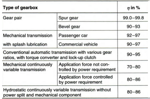
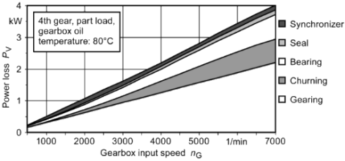
Flow inside Automotive Transmission Gearboxes
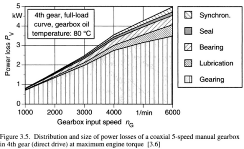
The lubrication system used in an automotive gearboxes are of dip-lubricated type or splash-lubricated gearboxes where the gears are partly immersed in oil and oil is transported to the tooth-meshing region while the teeth come out of the oil well. The rotation of gear teeth in highly viscous oil lead to drag known as churning power loss (category of load-independent power losses). Note that in real life, the two faces of gear teeth are in solid-to-solid contact which changes with time.
Thus, in order to apply the CFD method, some arbitrary gaps need to be assumed so that the two interacting teeth never touch each other (sometimes achieved by scaling down the driver and driven gears to 99.5% of their original sizes). It is recommended to start with 2D geometry where VOF multiphase model with dynamic meshing (smoothing, local- or global-remeshing and/or layering) to simulate the fluid flow for a pair of mating gears. Continuous variation of the geometry of the fluid volume during the operation, determined by the mating cycles of the gears, leads to high complexity in the simulation of fluid dynamics inside gearboxes, because it necessarily requires an update of the (distorted) mesh after a few time steps or fraction of degree rotation.
Another source of load-independent losses in gears is squeezing or pocketing generated due to variation of the volume between mating teeth thereby producing axial flows (squeeze effect) of the trapped lubricant. This loss is a lower order of magnitude when compared to churning losses.
Reference: "Automotive Transmissions: Fundamentals, Selection, Design and Application" by Giesbert Lechner, Harald Naunheimer
From STAR-CCM+ V2302 Release Notes: "In applications like gear box splashing droplets may break-up in smaller and smaller size until you can no longer model the very small droplets as Lagrangian particles. At the same time you still need to model the free surface of the bulk liquid. For such applications Mixture Multiphase with Large Scale Interface modelling (MMP-LSI) has become the method of choice. In general, MMP-LSI is relevant anywhere you have Volume Of Fluid (VOF) but that would be too expensive, and a mixture is present. But just like VOF, MMP-LSI comes at a comparably high cost if you can’t decouple the choice of flow time step from that needed to fulfil the small time step required for the volume fraction due to Courant (CFL) number constraints. To overcome this challenge we previously rolled out Implicit Multi-Step for VOF where simulations were typically sped up by 3-4x and in some cases by up to an order of magnitude."
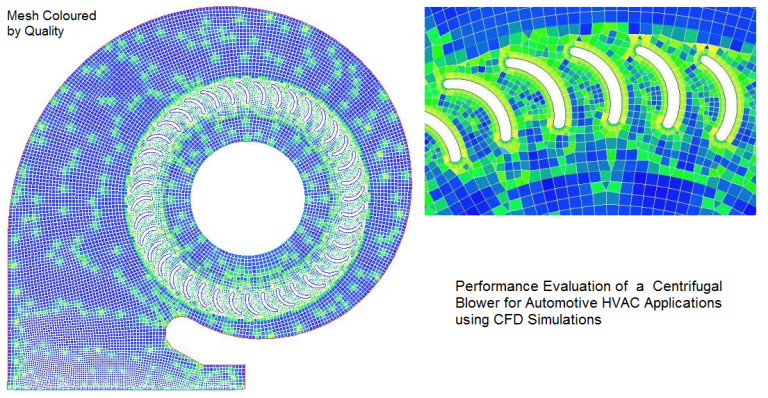
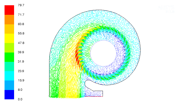
Flow inside a centrifugal blower for HVAC applications
Centrifugal blowers have far too many applications. Automotive HVAC is one of them. Following picture demonstrates typical layout of blower inside the heating module for automobiles. 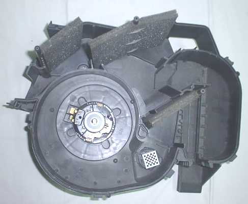
The purpose of this demonstration is:
- to gain insight into the operation of a centrifugal blower, effect of casing on pressure recovery
- develop an optimized throat shape, size and location
- execute basic optimization using 2D simulation
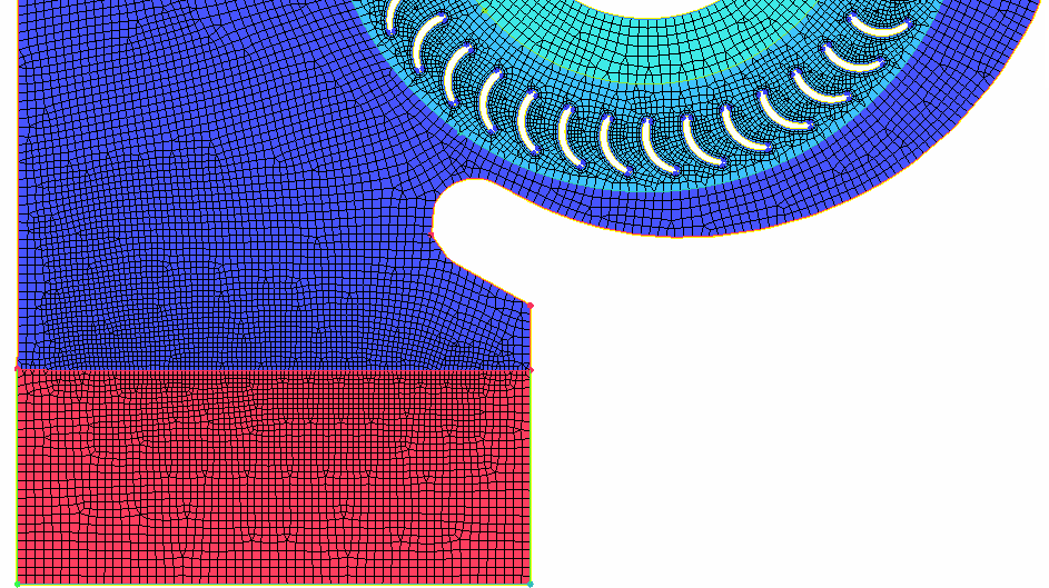
- use the 2D mesh to generate the 3D mesh, a novel use of mesh extrusion
- assess the improvement in results using Sliding Mesh Model (SMM) over Multiple Reference Frame (MRF) model
- study the effect of clearances between blade and casing on overall performance - 3D simulation
- check for the issues observed when solution for SMM is initialized with a converged MRF solution vs. full transient start where flow field is uniform.
- Incompressible air at 25 [°C] and 1 [atm] resulting in density of 1.185 [kg/m3.
- Realizable k-ε model with enhanced wall treatment
- Coupled solver with 2nd order discretization schemes for mass, momentum and turbulence
The results with Shear Stress Transport (SST) turbulence model is presented in following plots.
The plots Y+, velocity contour and wall shear on top wall are shown here.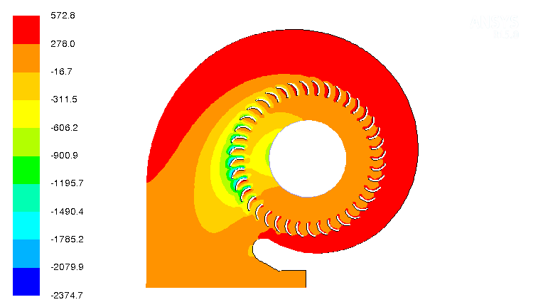
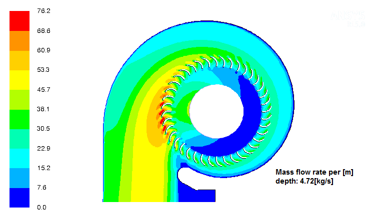
- The calculated mass flow rate per unit [that is 1 m] depth of the blade is 4.72 [kg/s].
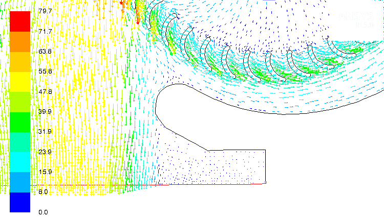
- Small level of reverse flow observed near the throat area which has been handles by redesign of this section and extending the outlet. Free-slip wall boundaries can be applied to eliminate the effect of extended domain.
- The location of throat is very close to the optimal design and there is no back flow into the blade cascade from the discharge region.
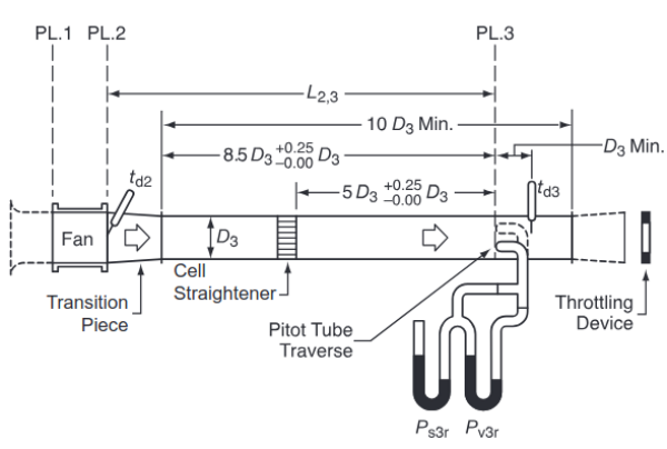
Testing of Fans
Cyclone Separators
- Cyclone separators are being used in industries for more than a century. This device falls under the category of what is called "Industrial Duct Collectors".
- Dust separation process utilize different methods ranging from fabrics (such as Air Cleaners in Automotive Intake Systems) to Electrostatic Precipitators in Coal-fired power plants
- Cyclone separators fall under the category of inertial separators which uses combination of the 3 most prevalent mechanical forces namely gravitational, centrifugal and inertial.
- In a cyclone, a high speed flow of fluid is established by tangential entry into a cylindrical geometry followed by a conical section.
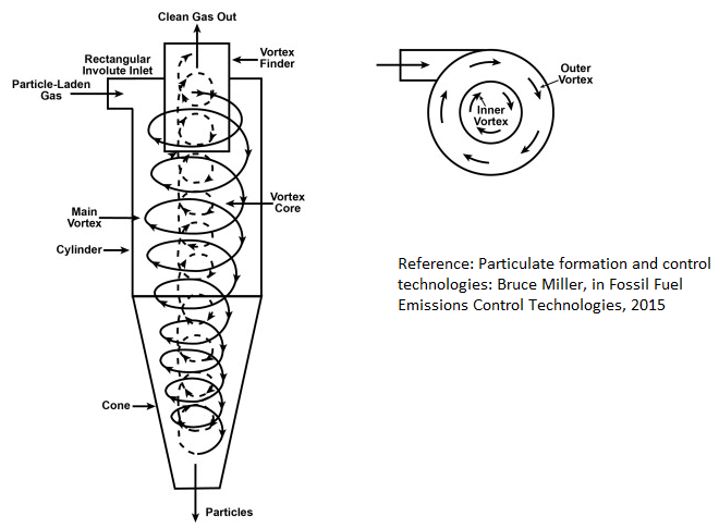
- The tangential entry of fluid stream result in a rotating and translating (swirling) pattern, beginning at the top and ending at the bottom conical end. Heavier particles in the rotating stream gets thrown out due to centrifugal forces and strike the outside wall, falling along the wall then to the bottom exit of the cyclone where they are collected.
- In the conical section, due to conservation of angular momentum, as the rotational radius of the stream is reduced, the tangential component of velocity is increased throwing out lighter and smaller particles, leading to separation of smaller particles, even up to size of 5 microns.
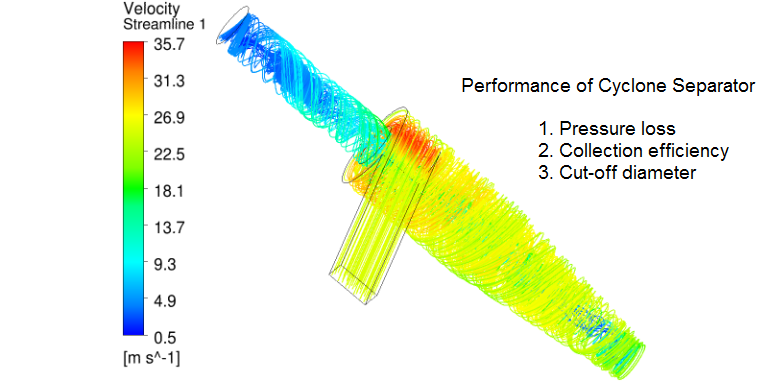
- [Reference: Particulate formation and control technology -- Bruce Miller, in Fossil Fuel Emissions Control Technologies, 2015] - The pressure loss and collection efficiency are two key performance parameters of this device. Cyclone separators are used for removing particles having diameters ≥ 10 [μm]. However, conventional cyclones seldom remove particles with an efficiency greater than 90% unless the particle size is ≥ 25 [μm]. High-efficiency cyclones can remove particles up to as los as to 5 [μm].
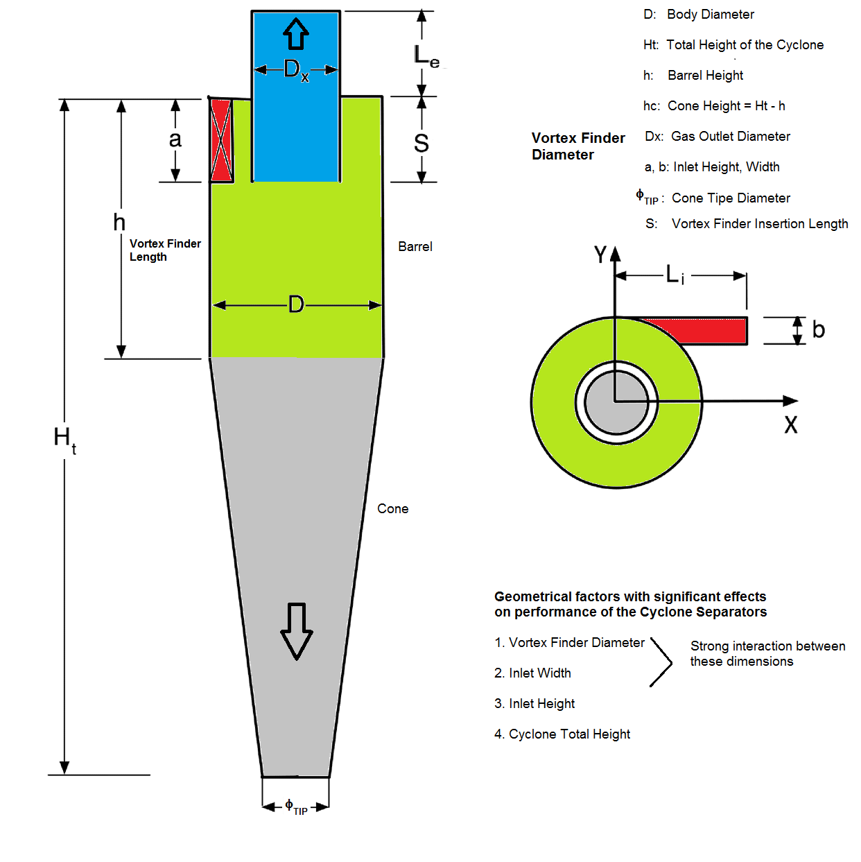
- A geometry of cyclone separator in STEP and IGES format can be are as available with the respective links. Dimensions in [mm] are Ht = 1250, D = 400, h = 500, S = 200, a = 200, Dx = 100.
- [Reference: Multiphase Flows in Cyclone Separators - Modeling the classification and drying of solid particles using CFD: Master of Science Thesis by Erik A. R. Stendal] Excerpts - When the swirling gas reaches the cone it will be accelerated due to the decreasing cross-sectional area and a vortex going upwards will form. This vortex will move inside the vortex finder and out through the gas outlet. The purpose of the vortex finder is to prevent contact between the inner vortex and the swirling gas in the barrel to prevent large pressure drops. The diameter of the vortex finder is an important parameter which affects the velocities in the barrel and, as a consequence, the total pressure drop of the cyclone. The particles injected into the cyclone separator will experience a centrifugal force towards the outer wall of the cyclone due to the swirling motion of the gas. The centrifugal force will be opposed by the drag force acting towards the core of the cyclone.
- The cut diameter of the cyclone is defined as the size of the particles collected with 50% collection efficiency. Collection efficiency is defined as the ratio of particles of a given size collected in the cyclone to the number of particles of that size entering into the cyclone at inlet.
- Despite such a long history of application in industry, the design principles so far as mostly based on empirical data. Recently, CFD techniques is being used to optimize the designs.
- 4 geometrical parameter which is tightly linked with the performance of cyclone separators are
- Vortex finder diameter
- Inlet width
- Inlet Height
- Total Height of the Cyclone
- The cone-tip diameter of the separator does not have noticeable effect on its performance.
Design Ratio: Cyclone Separator: The table below summarizes important dimensions of a cyclone separator. The range given are based on information found in reasearch and thesis documents. However, these dimensions are indicative only and are not intended to provide any engineering solutions.
| S. No. | Description | Design ratio | Typical range | |
| 1 | Cyclone diameter | 1.000 | - | |
| 2 | Diameter of vortex finder | 0.600 | 0.450 - 0.700 | |
| 3 | Dust outlet diameter | 0.300 | 0.250 - 0.350 | |
| 4 | Barrel height | 0.500 | 0.400 - 0.600 | |
| 5 | Height of the cone | 1.500 | 1.250 - 1.750 | |
| 6 | Vortex breaker cross height | 0.400 | 0.300 - 0.500 | |
| 7 | Height of the nozzle | 0.250 | 0.200 - 0.300 | |
| 8 | Nozzle width | 0.002 | 0.001 - 0.003 | |
| 9 | Vortex breaker cone height | 0.125 | 0.100 - 0.150 | |
| 10 | Diameter of vortex breaker cone | 0.250 | 0.200 - 0.300 |
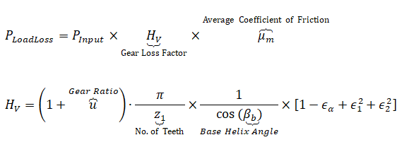
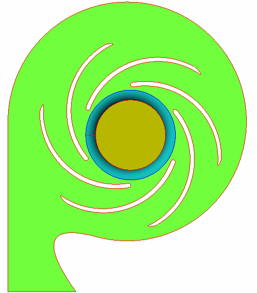
Gear Pumps
Gear pumps with involute profile of Gerotor type and lobe pumps are two category of devices which require a dynamic mesh motion to solve the flow field.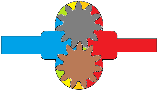
- PInput = input power to drive gear
- εα = transverse contact ratio
- ε1 = addendum contact ratio
- ε2 = dedendum contact ratio
- grease lubrication - applied in low speed / low load applications with tangential speed < 5 [m/s]
- splash lubrication (oil bath method) - used with an enclosed system. The rotating gears splash lubricant onto the gear system and bearings. It needs at least 3 [m/s] tangential speed to be effective.
- forced oil circulation lubrication: there are many methods, one of them is the oil drop method where an oil pump is used to suck-up the lubricant and then directly drop it on the contact portion of the gears via a delivery pipe.
Centrifugal Pumps
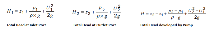
- z [m] = height of the measurement plane with respect to arbitrarily chosen datum plane
- U [m/s] = mean (area-average) velocity at pressure measurement planes
- ρ [kg/m3] = density of fluid
- p [Pa] = static pressure (the value should be consistent at outlet and inlet: either both in gauge pressure or both in absolute pressure
- g [m/s2 = 9.806 - acceleration due to gravity
- N [RPM] = rotation speed of impeller in revolutions per minute
- ω [rad/s] = rotation speed of impeller
- Q [m3/s] = volumetric flow rate through the pump (each eye)
Fan Laws: applicable when the efficiency of scaled model and actual model are assumed nearly equal.

Measurement uncertainty for the individual operating parameters: reference - www.ksb.com/centrifugal-pump-lexicon/total-tolerance/191302
| Variable | Symbol | Class 1 [%] | Class 2 [%] |
| Volume flow rate | tQ | ± 4.5 | ± 8.0 |
| Pump discharge head | tH | ± 3.0 | ± 5.0 |
| Pump efficiency | tη | -3.0 | -5.0 |
Sample Pump Performance Curve
Note the constant efficiency lines - can you explain what will be the impact of increase in impeller diameter on efficiency for a given flow rate?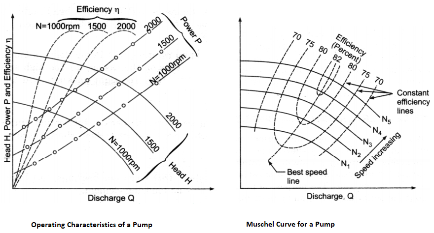
Sample design data of a centrifugal pump [Reference: 1Numerical 3D RANS simulation of gas-liquid flow in a centrifugal pump with an Euler-Euler two-phase model and a dispersed phase distribution: T. Mueller, P. Limbach, R. Skoda, 2Investigation of the handling ability of centrifugal pumps under air-water two-phase inflow: model and experimental validation: Qiaorui Si et al.]
| Performane / Design Parameters | Symbol | Unit | Value1 | Value2 |
| Impeller inlet diameter | d1 | [mm] | 260 | 79 |
| Impeller inlet duct diameter | di | [mm] | - | 65 |
| Blade inlet width | b1 | [mm] | 46 | - |
| Impeller blade inlet angle | β1 | [°] | 19 | - |
| Impeller outlet diameter | d2 | [mm] | 556 | 140 |
| Blade outlet width | b2 | [mm] | 46 | 15.5 |
| Impeller blade outlet angle | β2 | [°] | 23 | - |
| Blade thickness | s | [mm] | 12 | - |
| Shape of blades | - | [-] | 2 circular arcs | Archimedes' spiral |
| Number of blades | z | [no.] | 5 | 6 |
| Nominal flow rate | Q | [m3/s] | 0.114 | 0.014 |
| Nominal pump head | H | [m] | 10.16 | 20.2 |
| Nominal rotational speed | ω | [rad/s-1] | - | 305 |
| N | [RPM] | 540 | 2910 | |
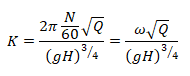
| Specific speed | Ns | [s-1] | 32 | - |
Losses in Pumps
Slip Losses: The losses due to "imperfect guidance of the flow by the blades" or slip due to fluid not following the solid rotating wall and fluid. As the fluid traverses through the impeller blades the pressure between each adjacent blade (pressure side of one blade and suction side of other blade) will be different due to the adverse tangential or peripheral pressure gradient. This results in a secondary circulation which forces the fluid exiting the blade to flow backward (from tip towards the hub) with respect to the rotational direction of the impeller. To reduce slip losses, it is suggested to increase the inlet blade angle and reduce the outlet angle (Sixsmith). The slip at shut-off head is a measure of the drag (or 'hold') which the blades have on the fluid (Crewdson). The increase in number of blades reduces slip loss but increases frictional loss At the same time, number and spacing of the blades are strongly related to the diameter of the impeller and and the size of the side channel (height of the blades along axial direction).
Shock Losses: Also known as incidence losses, these losses occur at the entry to the blades and predominantly at off-design operating conditions. It is believed that the difference in angle between the blade and the velocity of fluid entering the blade results in difference of angular momenta between the slower moving fluid in the channel and the faster moving fluid in the impeller. The shock effect is quantified as the ratio of the mean peripheral (tangential) fluid velocity at the blade inlets to the velocity of the blade (at the inner diameter of the blades). As the losses from shock and slip are mainly due to misalignment of the blade and fluid angles, these could be minimised by increasing the impeller diameter and decreasing the hub diameter (Raheel and Engeda).
Cavitation in Pumps
Cavitation refers to localized boiling of evaporation of any liquid due to reduction in static pressure below its vapour pressure at its operating temperature. However, the phenomena is almost always associated with formation and collapse of bubbles as they move along the mean flow path. A liquid increases its volume significantly when it vapourizes. 1 m3 of water at room temperature becomes 1400 m3 of vapour at the same temperature and pressure. The calculation is as follows (assuming water vapour to behave like an ideal gas):- Mass of 1 m3 of water at 20 [°C] = 998.2 [kg]
- Gas constant for water vapour = 8134/18 =451.9 [J/kg-K]
- Volume occupied by water vapour at 20 [°C] and 1 [bar], V = mRT/p = 1360 [m3].
- However, the density ratio of water liquid and vapour is 998.2 [kg/m3] / 0.0173 [kg/m3] = 57655.
Another term associated with cavitation phenomena is NPSH (Net Positive Suction Head). NPSH is the difference "total pressure at pump inlet" - "vapour pressure of liquid at operating temperature" expressed as head of that fluid. That is:
ρ × g × NPSH = P0 - Pv. Note that total (or stagnation) pressure and not the static pressure is used in calculation.
NPSH is further differentiated in two types: NPSHREQUIRED or NPSHr and NPSHAVAILABLE or NPSHa. The former is supplied by pump manufacturers and this refers to the NPSH that must be available at impeller eye. Hence this value must be independent of the the system in which pump is installed and should solely depend on the design (shape and size) of the pump.
- NPSHr indicates the lowest inlet pressure required by the pump at a given flow to avoid cavitation and is independent of the kind of liquid pumped.
- As the liquid flows from the pump inlet port (suction port) to the eye of the impeller, the velocity increases and hence pressure decreases.
- Additional pressure losses occur due to shock and turbulence as the liquid strikes the impeller. The centrifugal force of the impeller vanes further increases the velocity and decreases the pressure of the liquid.
- Cavitation zone predominantly occurs near the suction side of the leading edge of the impeller blades.
- In CFD simulations, the volume fraction plots on the impeller blades can be used to estimate the extent of cavitation.
- CFD simulation for cavitation is primarily a multiphase flow simulation where the volume fraction on non-condensible air can be specified in the range 1 ~ 5 [ppm]. Note that the amount of O2 dissolved in water at atmospheric pressure at 15 [°C] is approximately 10.0E−6 [g/g]. For N2, this value is about 15.0E−6 [g/g]. However, the solubility of air in water is not the sum 25.0E−6 [g/g].
- The solubility of O2 in water is higher than the solubility of N2. Air dissolved in water contains approximately 36% O2 compared to 21% in air.
- Lower the NPSHr, higher the suction capacity.
- On the other hand, NPSHa is dependent on the overall system (supply tank or sump) to inlet to the impeller eye.
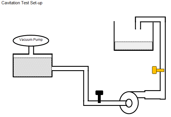
In manufacturer's catalogues, characteristic curves (Δp-Q curve) of a pump also contain a curve for NPSHr vs. Q. The NPSHr values indicated are based on measurements carried out with cold water as pumping liquid. NPSHr is also referred to as NPSH3 per API 610 and determines the operating point at which a pump will operate at 3% loss of head due to cavitation. In test set-up, the pump is installed with a starving device (flow and pressure regulator) on its suction line so that the test loop can deliver variable NPSHa. Cavitation begins as small bubbles before any indication of loss of head or capacity can be observed. This is called the point of incipient cavitation and corresponding head is denoted by NPSHi. NPSHr ≈ [2 ~ 20] × NPSHi, is sole responsibility of the pump manufacturer.
Excerpts from "Understanding Centrifugal Pump Curves" by MGNewell: Generally speaking NPSHr does not vary dramatically between variations in impeller trim which is why we do not see separate curves for the minimum and maximum impeller trims. Those curves are actually present, but they are overlaid by the design trim NPSHr curve.Reference - www.iso.org/standard/41202.html: ISO 9906:2012 specifies hydraulic performance tests for customers' acceptance of rotodynamic pumps (centrifugal, mixed flow and axial pumps). It is intended to be used for pump acceptance testing at pump test facilities, such as manufacturers' pump test facilities or laboratories. It can be applied to pumps of any size and to any pumped liquids which behave as clean, cold water. It specifies three levels of acceptance:
- grades 1B, 1E and 1U with tighter tolerance
- grades 2B and 2U with broader tolerance
- grade 3B with even broader tolerance
NPSH: Net Positive Suction Head
CFD simulations can be used to determine NPSHr by running a series of simulations for a given system and determining when the performance exhibits 3% head loss. For accurate predictions, the effect of vapor formation and collapse (cavitation) and Non-Condensable Gases (NCG) such as dissolved oxygen should also be considered.
The dimensionless parameter that governs the cavitation characteristics of a centrifugal pump is cavitation number described below.
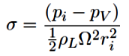
- ρL = density of liquid
- pi = inlet pressure at pump suction port (Pa)
- ri = impeller tip radius (m)
- Ω = pump rotation speed (rad/s)
- pV = vapour pressure or saturation pressure at working temperature of the liquid
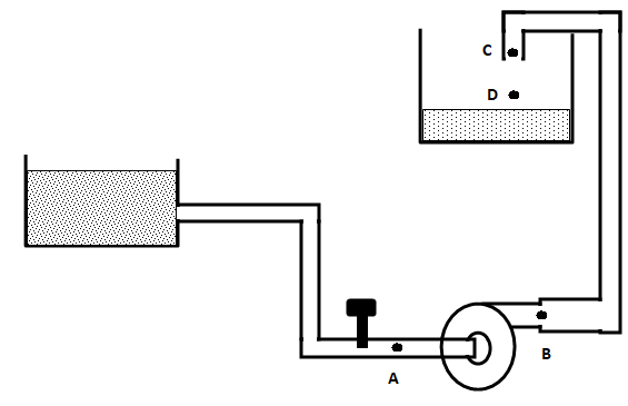
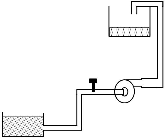
Refer to the two operating conditions of a pump at same flow rates, pipe diameters, elevation of discharge tanks and water levels in supply tanks. Should the NPSHREQUIRED be different in the two situations? Would the NPSHAVAILABLE be same in both of the scenarios?
Cavitation Test
Refer to the graph below how NPSHr and NPSHa varies with respect to flow rate in the pump. 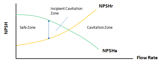
Effect of Non-condensible Gases
Air (hence O2 and N2) are soluble in water, though at very low level. Still, they are good enough to keep species under water alive. Similarly, the operating liquids in most of the industrial applications have small amount of non-condensible gases present. These can be in dissolved state or mixed with liquid due to leakage / aeration.- The primary effect of non-condensible gas is due to the expansion of gas at low pressures. This can lead to significant values of local gas volume fraction causing considerable change in density, velocity, viscosity and pressure distributions.
- The secondary effect of a non-condensible gas is on the early inception of cavitation by increasing the number of nucleation sites for bubble formation.
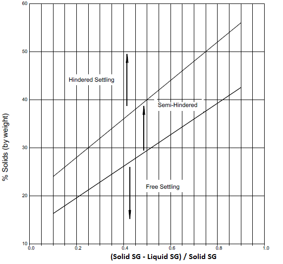
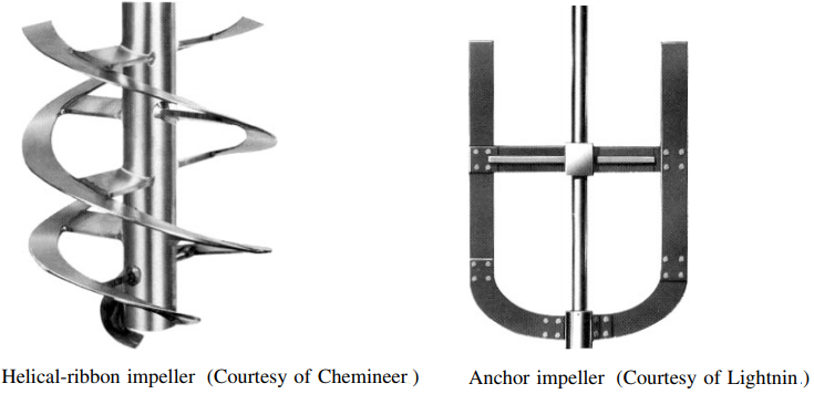
Mixing Tanks or Stirred Tanks
Also known as mechanically agitated tanks, these are widely used in the process (pharmaceutical, beverage...) industries for mixing of single or multiphase fluids. "Mixing time" is one the most critical performance parameter which is defined as the time to achieve complete homogenization of injected tracer (fluid) or time to mix reactants fed into a tank. The mixing process simulation does not account for Agglomeration which the phenomena of combining of finely dispersed particles into larger parcels, usually caused by a re-arrangement of surface forces resulting from a change of environment. 
The time of homogenization (mixing time) is defined as the time from the introduction of the tracer to the time when the tracer concentration at the probe position reaches and remains within a certain range of the final value. If the range is set to ± 5% it is designated as t95.
Flash Mixer: An agitator used to mix a small amount of additive into a continuous stream where the Residence Time is extremely short. Residence Time it average time a process component remains in the mixing environment in a continuous process.
Mixing process needs to handle both the immiscible (e.g. water - silicone oil, water - benzene) and miscible liquids (e.g. water - alcohol, water - caustic solution), liquid with large difference in viscosities (e.g. water-0.001 Pa.s and molasses-2 Pa.s) and fluids with large difference in densities. In case of miscible liquids, only transient simulation can be performed and mass or volume fraction of one the phases needs to be monitored at different locations of the tank. If left for a long enough period of time, miscible liquids will any way dissolve in one another and form a homogeneous solution. A sliding mesh model is recommended to transport the velocity of the impeller to the bulk liquid in the stationary domain.
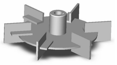
Rushton Turbine
Reference: Hayward Gordon - MASTERING MIXING FUNDAMENTALS: A technical guide from the experts in the industry - Blending:blending of miscible fluids. If left for a long enough period of time, miscible liquids will dissolve in one another and form a homogeneous solution. The majority of liquid/liquid blending applications fall into this category. Applications involving immiscible (insoluble) fluids are classified as dispersion applications which involves very different mixer sizing methods.
There are other types of mixtures known as static mixtures where the mixing elements are inserted in the pipelines and the liquids mix as they flow through them. Kenics static mixer from Chemineer is one such device.
Reference: Mechanical Design of Mixing Equipment, D. S. DICKEY, MixTech, Inc. J. B. FASANO Chemineer, Inc - Dry-solids mixers are normally applied to flowable powdered materials. The action of the mixers can be categorized as summarized below.
- Tumble mixers
- Convective mixers which use a ribbon, paddles, or blades to move material
- High-shear mixers which create a crushing action like a mortar and pestle
- Fluidized mixers as in fluidized beds and
- Hopper mixers which use discharge and recirculating flow to cause mixing
The Reynolds number for agitators or mixers are calculated based on blade tip speed. However, the adopted formula has been simplified a bit by dropping π and the formula is Re = ρ[kg/m3]×N[rev/s] ×D[m2]/μ [Pa.s]. Flow is assumed turbulent when Re > 10,000 ((McCabe, Unit Operations of Chemical Engineering, 1993). Torque per Equivalent Volume [Torque on impeller / Working Volume of Tank] is an extremely useful ratio which is used as the basis for mixer sizing and describes the level of mixing for any application.
Vapour Pressure of Water
| T [°C] | PSAT [Pa] | 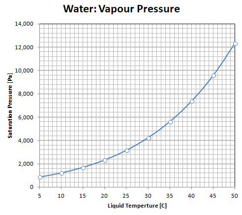 |
| 5 | 872.60 | |
| 10 | 1228.1 | |
| 15 | 1705.6 | |
| 20 | 2338.8 | |
| 25 | 3169.0 | |
| 30 | 4245.5 | |
| 35 | 5626.7 | |
| 40 | 7381.4 | |
| 45 | 9589.8 | |
| 50 | 12344 | |
| 55 | 15752 | |
| 60 | 19932 | |
| 65 | 25022 | |
| 70 | 31176 | |
| 75 | 38563 | |
| 80 | 47373 | |
| 85 | 57815 | |
| 90 | 70117 | |
| 95 | 84529 | |
| 100 | 101320 |
Surface Water: water on the earth’s surface, including rivers, ponds, water reservoirs (dams), springs, creeks and wetlands/swamps. Most surface water comes from rainfall (precipitation) run-off from the surrounding land area (catchment). Surface water also includes the solid forms of water - snow and ice.
Non-Surface Water: water under the earth’s surface, underground water, aquifer system. It also includes soil water.
Propellers
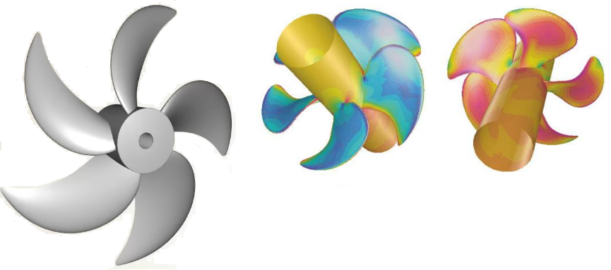
In other words: The 'face' of a blade is the high-pressure side or pressure face of the blade. This is the side that faces aft (downstream) and pushes the water when the vessel is in forward motion. The 'back' of the blade is the low pressure side or the suction face of the blade. This is the side that faces upstream (incoming water) or towards the front of the vessel.
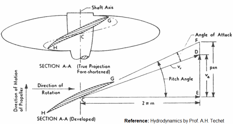
Propellers are axial flow type. In most of the rotating devices and especially in axial flow machines, blades have two edges: leading edge and trailing (lagging) edge. The blades rotates in the direction formed by rotating trailing edge towards the leading edge. The shape of the blades have speacial twist and the parameters defining the twists are known as rake, skew and pitch.
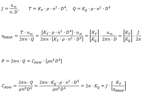
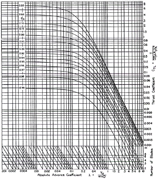
Propellers operate in non-uniform flow field (wake regions) created by the boat or ship body. However, the theoretical studies of the performance of an impeller is carried out in calm water known as open-water characteristics. Advance ratio, thrust coefficient, torque coefficient and power coefficient are the key parameters required to define a propeller.
- u∞ = ship or flight (free-stream) velocity
- us = ship velocity
- ρ = density of the liquid
- n = revolution per second (RPS)
- D = propeller tip diamter
- T = Thrust
- Q = Torque
- P = Power
- J = Advance ratio or advance number
- KT = thrust coefficient
- KQ = torque coefficient
- ηPROP = propeller efficiency
- ηt = propulsive efficiency
- CPOW = power coefficient
- Rt = total ship resistance
- w = wake fraction
- t = thrust deduction factor
Input
- Thrust, T = 2,000 [N]
- Boat speed, u∞ = 5[m/s] = 18 [km/hour]
- Fluid Density, ρ = 1000 [kg/m3]
- Propelle blade tip diameter, D = 0.75 [m]
- RPS, n = 20 [rev/s]
- Number of blades, nB = 4 [ - ]
Step-1
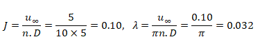
Calculate ideal (actuator disc) efficiency, CT
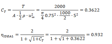
Step-2
Calculate advance ratio, J
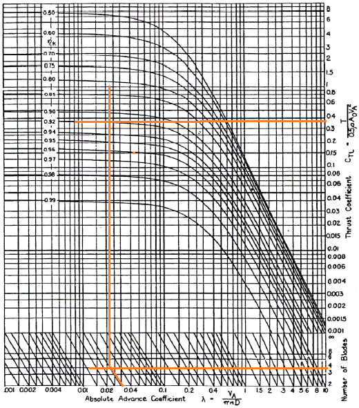
Step-3
From Kramer diagram, calculate the propeller efficiency.
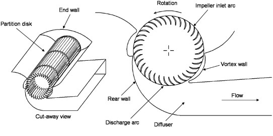
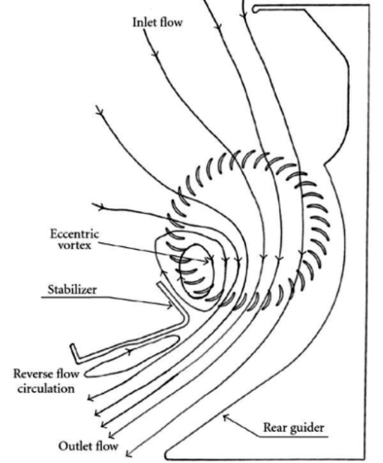
Cross-flow Fans
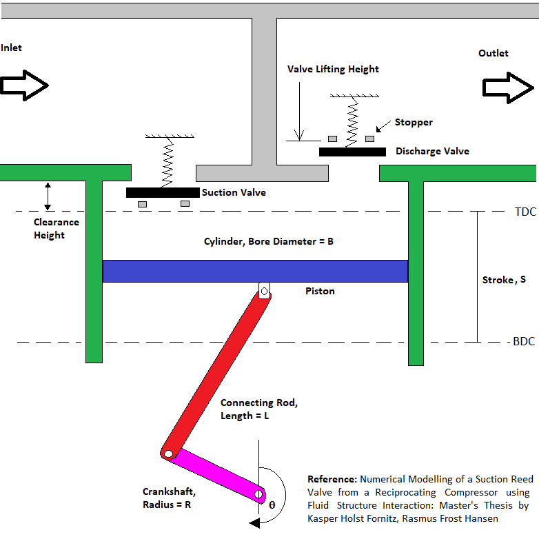
Reciprocating Compressors
Types of Hydraulic pumps
- Hydrodynamic: a rotating element within a casing imparts radial velocity to the fluid which exits in a discharge nozzle
- Hydrostatic: also known as positive displacement pumps, displace a fixed volume of fluid per cycle (rotation of shaft)
- Rotary: a rotating vane, screw or gear collects fluid in its void on the suction side of the pump and forces it to the discharge side
- Reciprocating: fluid is pulled into a void on the suction side of the pump and then pushed during the compression stroke, through the discharge port of the pump.
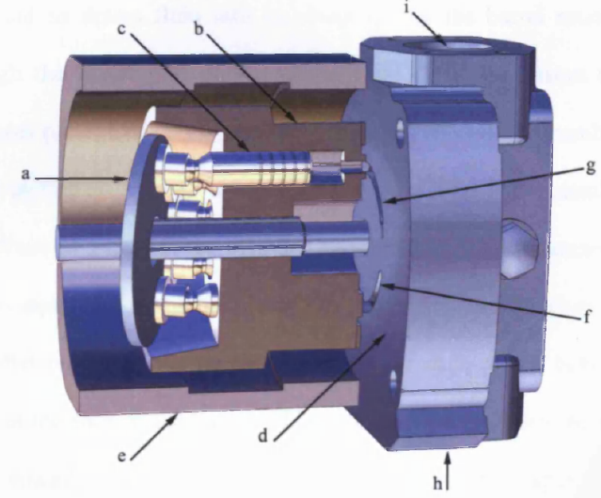
Swash-plate axial piston pump
Reference: Axial Piston Pump - Leakage Modelling and Measurement, PhD Thesis by Jonathan Mark Haynes
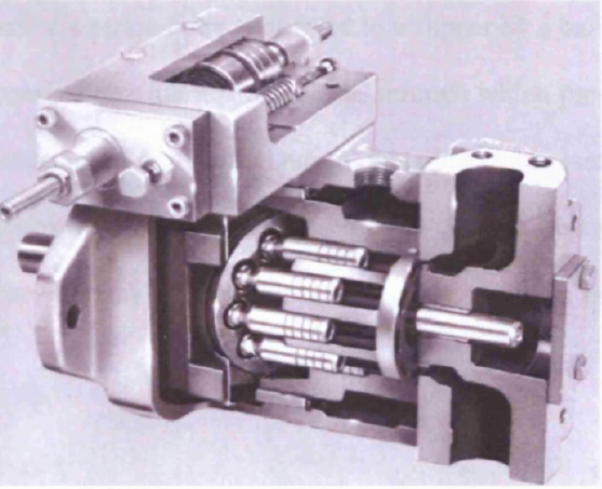
Reference: Use of CFD Technology in Hydraulics System Design for off-Highway Equipment and Applications by Shivayogi S. Salutagi, Milind S. Kulkarni and Aniruddha Kulkarni - International Journal of Materials, Mechanics and Manufacturing, Vol. 4, No. 1, February 2016
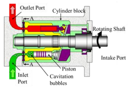
Leakage Paths:
- The gap between the rotating barrel and fixed port plate introduces a cross-port leakage and a leakage across the barrel edges to the internal casing, and ultimately back to tank.
- The slipper face consists of a lubrication orifice, through which pressurised fluid can flow, ultimately returning back to tank.
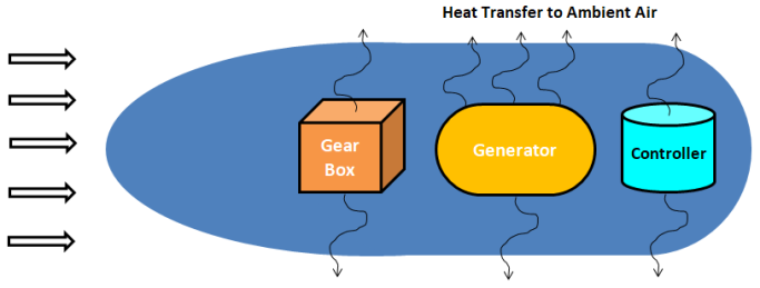
Wind Turbines
Wind Turbines (sometime also referred as WTG: Wind Turbine Generator) are a set of device where one rotating system (Nacelle) contains many other rotating systems inside it (generator, gear-box...). A simplified evaluation of heat transfer capacity of a nacelle housing can be performed as described below.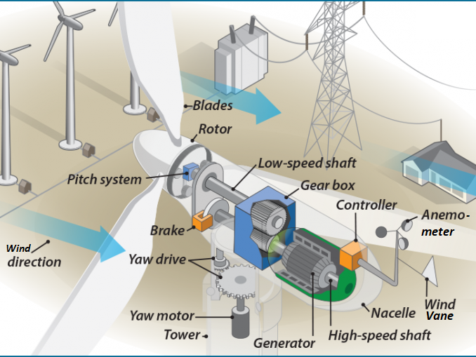
Wake Modeling
Excerpts from "Wind turbine wakes modeling and applications: Past, present, and future" by Li Wang et al, Ocean Engineering Volume 309, Part 1:- The wake effect refers to the phenomenon where natural wind, after passing through a Wind Turbine, converts part of its energy into mechanical energy, resulting in reduced wind speed, increased turbulence, and wind shear.
- Studies indicate that the wake effect can lead to power losses of 10 ∼ 40% in wind farms and significantly increase the fatigue load on downstream WTs (Fei et al. 2020 and Cai et al. 2021).
- Wind tunnel experiments and field measurements constitute the primary methods for wake investigations. Wind tunnel experiments, based on similarity theory, reveal the flow field dynamics of wind turbines and wind farms, providing critical insights into the flow field structure of Wind Turbine in boundary layer flows (Bottasso et al. 2020).
WAsP: some excerpts from official website - Wind Atlas Analysis and Application Program - used to simulate wind flow over terrain and estimate the long-term power production of wind turbines and wind farms. Can be used for sites located in all kinds of terrain. WAsP contains the PARK2 and PARK1 wake models for calculation of wind farm wake effects. WAsP includes two high-resolution microscale wind flow models for vertical and horizontal extrapolation of the wind climate. PyWAsP is a python-based API for running WAsP and WAsP Engineering models. Turbulence intensity data from wind measurements at a nearby meteorological mast can be used for correction of modelled turbulence intensity.
As per "Wind Farm Site Selection Using WAsP Tool for Application in the Tropical Region" by Kamdar et al. -- WAsP uses a linear model composed of a comprehensive collection of individual modules according to the physical characteristics of flows in the planetary boundary layer to predict the vertical and horizontal extrapolation of wind. The WAsP flow model requires the following inputs: (1) Terrain height, (2) surface roughness, and (3) obstacle effects also known as the wind atlas methodology.The user guide or tutorial examples for latest releases are not available to public. As per WAsP version 11 on-line documentations published in 2014, the WAsP methodology consists of five main calculation blocks:
- Analysis of raw wind data
- Generation of wind atlas data
- Wind climate estimation
- Estimation of wind power potential
- Calculation of wind farm production
Known limitations: as per version 11
- WAsP uses a default air density of 1.225 [kg/m3] (which corresponds to standard pressure and 15 °C temperature) when calculating power density unless you specify the air density in the project's parameters. Similarly, power production is calculated for this standard air density if one of the sample power curves is used. You can change the air density in the project parameters; this will affect power density, but not AEP calculations.
- Only if the power curve is specified for the actual site air density, or an existing power curve has been scaled to the site air density (this is only recommended for some turbines though), will the wind turbine power production calculated by WAsP correspond to this air density. In 'real' projects it is strongly recommended to obtain a site-specific power curve from the manufacturer of the wind turbine.
Openwind: A "Wind Farm Modeling and Layout Design" tool that takes into account wind resources, wakes, noise, shadow flicker, curtailments, GIS constraints... It optimizes layouts and turbine positions to minimize the cost of energy, taking into account energy production, operations and maintenance costs and capital costs including turbine and plant development costs.
PyWake is an open-sourced and Python-based wind farm simulation tool developed at DTU capable of computing flow fields, power production of individual turbines as well as the Annual Energy Production (AEP) of a wind farm. The repository has 64 directories, 716 files excluding few files related to installation. The list of directories and files can be found in this text file.
OpenFAST is a National Renewable Energy Laboratory (NREL) supported, open-source physics-based tool for simulating wind turbine aero-elasticity, control, and structural dynamics. OpenFAST is a wind turbine simulation tool which builds on FAST v8. FAST.Farm extends the capability of OpenFAST to simulate multi-turbine land-based, fixed-bottom offshore, and floating offshore wind farms. The list of directories and files can be found in this text file.
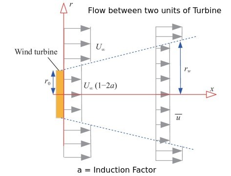
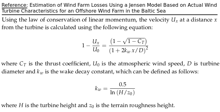
Jensen Empirical Model for Wake in Wind Farms: also known as 'Park' model. The main factor in Jensen model is Wake decay coefficient (determines how quickly ambient air mixes into the wake) which is decided by turbulence intensity. Jensen models is derived based on linear expanding wake assumption. A simple Python code to implement Jensen formula for estimation of power output from a wind farm can be accessed here. This is based on power-curve described below.
Reference: "Best Practices for Wake Model and Optimization Algorithm Selection in Wind Farm Layout Optimization"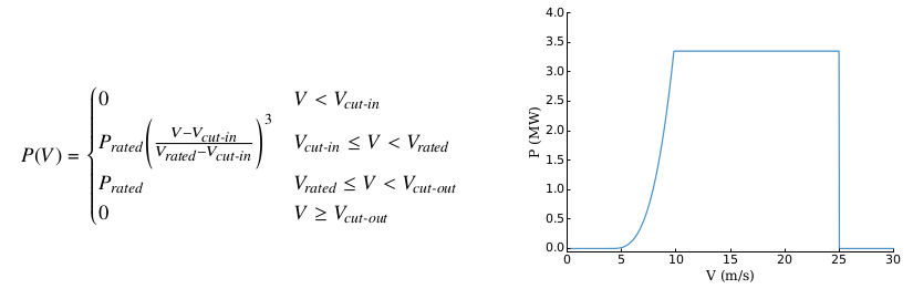
A multi-objective cost-power formulation is required for optimal placement of wind turbines (determination of number of turbines and their positions - also known as Micro-Siting of Wind Turbines) towards achieving the target of maximization of power (AEP: Annual Energy Production) and minimization of cost which requires consideration of wake effects. Wind farm analysis software is required for real-time monitoring of power exchange between wind turbines and the power grid.
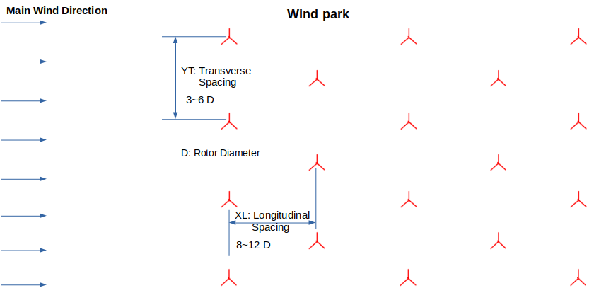
Not only the wake effect, the distance to the nearest residential building is important to not disturb the inhabitants by noise emission and shadow flickering of the turbine.
"Wake modeling and simulation" by Gunner C. Larsen et al.: The downstream advection of a wake from the emitting turbine describes a stochastic pattern known as wake meandering. It appears as an intermittent phenomenon, where winds at downwind positions may be undisturbed for part of the time, but interrupted by episodes of intense turbulence and reduced mean velocity as the wake hits the observation point. Summary of wake models can be found in this document.
"The revised FLORIDyn model: implementation of heterogeneous flow and the Gaussian wake" by Marcus Becker et al. "FLORIS and FLORIDyn are parametric models which can be used to simulate wind farms, evaluate controller performance and can serve as a control-oriented model." FLORIS model (FLOw Redirection and Induction in Steady state), Gebraad et al. FLORIDyn model: FLOw Redirection and Induction Dynamics - "The Flow redirection and induction dynamics model allows for the dynamic simulation of FLORIS wakes under heterogeneous conditions. Such conditions are changing wind speeds, directions, and ambient turbulence intensity over time and space. The model also includes wake interaction effects and an added turbulence model."Simulator for Offshore Wind Farm Applications (SOWFA) is an NREL-developed high-fidelity, CFD-based wind farm simulation tool built on OpenFOAM. It models wake dynamics using Actuator Line (ALM) or Actuator Disk (ADM) models to simulate turbine-flow interaction, wake propagation, and deflection within turbulent Atmospheric Boundary Layers (ABL).
NREL 5 MW Reference Wind Turbine: Definition of a 5 [MW] Reference Wind Turbine for Offshore System Development by J. Jonkman, S. Butterfield, W. Musial, and G. Scott
| Rating | 5 MW |
| Rotor Diameter | 126 m |
| Hub Height | 90 m |
| Drivetrain | High-speed, multiple-stage gearbox |
| Minimum, Rated Rotor Speed | 6.9 rpm, 12.1 rpm |
| Cut-In, Rated, Cut-Out Wind Speed | 3.0 m/s, 11.4 m/s, 25 m/s |
| Overhang, Shaft Tilt, Pre-cone | 5.0 m, 5.0°, 2.5° |
| Rotor Mass | 110,000 kg |
| Nacelle Mass | 240,000 kg |
| Tower Mass | 347,460 kg |
| Coordinate Location of Overall CM | (-0.2 m, 0.0 m, 64.0 m) |
Enercon E–18 wind turbine specifications
| Rotor Diameter | Hub Height | Cut–In Speed | Cut–Out Speed | Survival Wind Speed | Rated Power | Rated Wind Speed |
| 18 m | 28.5 m | 2.5 m/s | 25.0 m/s | 67.0 m/s | 80 kW | 12.0 m/s |
Betz Limit: Albert Betz determined in 1919 that a wind turbine can extract at most 59% of the energy that would flow through the cross section of the turbines. The Betz limit applies regardless of the design of the turbine. More recent work by Gorlov shows a theoretical limit of about 30% for propeller-type turbines. Actual efficiencies range from 10% to 20% for propeller-type turbines, and higher up to 35% for three-dimensional vertical-axis turbines like Darrieus or Gorlov turbines.
Lifecycle of a Wind Farm:
Site Identification and Screening > Wind Resource Assessment > Environmental and Regulatory Approvals > Micro-siting and Layout Optimization > Turbine Selection > Engineering and Design > Financial Modeling and Investment > Procurement and Construction > Grid Connection > Commissioning > Operations and Maintenance > Power Generation and Supply > Performance Optimization.Main risks to wind farms are: (1) Poor wind resource estimation (2) Grid constraints and/or curtailment and (3)Wake losses due to non-optimal layout
Wind resource assessment (WRA) is the process of estimating the wind power potential around an area. The output usually is wind resource map showing the variation of the mean wind speed or power density over that area , for a given height above ground level.The wind speed distributions combined with the power curve of chosen wind turbines is used to obtain power production map. Another output from WRA is the wind direction probability distribution (wind rose) which shows the frequency distribution of wind directions.To decide siting of individual wind turbines, an assessment is carried out as per IEC 61400-1. This provides estimates for each wind turbine site of the 50-year extreme wind, shear of the vertical wind profile, flow and terrain inclination angles, free-stream turbulence, wind speed probability distribution and added wake turbulence.
Wind Power Density [W/m2]: A measurement used to assess wind energy potential in an area, often categorized from Class 1 (poor) to Class 7 (superb). IEC categorizes wind environment based on average annual wind speed: the categories named Class I, II, III and IV are assigned to average annual wind speeds 10 [m/s], 8.5 [m/s], 7.5 [m/s] and 6.0 [m/s] respectively. International Electrotechnical Commission (IEC) also sets standards for the wind speeds each wind class must withstand.
Wind power density (strictly speaking power flux) is the maximum available wind power per unit area expressed as P = ½·ρ·v3 and is divided into seven categories on the basis of wind speed and annual wind power density.| Class of Wind Power | Range of Mean Wind Speed [m/s] | Wind Power Density [W/m2] | Resource Potential |
| 1 | 3.5 - 5.6 | 50 - 200 | Poor |
| 2 | 5.6 - 6.4 | 200 - 300 | Marginal |
| 3 | 6.4 - 7.0 | 300 - 400 | Fair |
| 4 | 7.0 - 7.5 | 400 - 500 | Good |
| 5 | 7.5 - 8.0 | 500 - 600 | Excellent |
| 6 | 8.0 - 8.8 | 600 - 800 | Outstanding |
| 7 | > 8.8 | > 800 | Superb |
The Levelized Cost of Energy (LCOE) is elaborated as a measure of the average net present value of the generated electricity for a particular system over its lifespan. LCOE = "Average total cost to build and operate a power plant over its lifetime" / "Total power generated by the power plant over that lifetime". The capacity factor of the wind turbine is defined as the dimensionless ratio of the "average power output" and the "rated power output" over a certain period of time (usually over one year).
Meteodyn Forecast is a wind power production forecasting service coupled with a web application for monitoring and visualizing the generated data. Output is very short-term such as minutes, hours or short-term such as days, weeks or mid-term: months, seasons. Additional output includes "wind speed and direction" and "production probability distribution" such as P10, P25.
Wind Modeling Approaches: (1) Time-Series Method - Use measured hourly wind data, Compute power at each time step, Aggregate energy. Assumes steady-state wind at each time step. (2) Statistical Method (Weibull Distribution) - requires Shape parameter (k) - a dimensionless value between 1 and 3, Scale parameter (A) in [m/s], Integrate turbine power curve (turbine manufacturer power curves) over distribution.
The two–parameter Weibull probability distribution is frequently used in calculations to describe the wind speed histogram. The probability distribution function (PDF) of Weibull distribution is defined as: f(u) = [k/A] * (U/A)k-1 * e-(u/A)k. Weibull shape parameter k describes the variations of wind speed where small values of k shows higher variations in wind variables and large values of k indicate a rather constant wind speed. Corresponding cumulative probability function (integral of the PDF with respect to speed) for the Weibull distribution can be expressed as F(u) = 1 - e-(u/A)k.P50 represents the median estimated energy yield. It is the level of energy production that has a 50% probability of being exceeded (projected to surpass 50% of the time throughout the lifespan of the project) and a 50% probability of not being reached over a given period, typically a year. P90 is a more conservative estimate (90% probability of being exceeded) often used by banks and investors for financing to manage risk. The MWhr value for P90 will be lower than MWhr value for P50: P90 = P50 - 1.282 × σ where the total uncertainty = σ. Similarly, P75 = P50 - 0.6745 × σ where 1.282 and 0.6745 are standard normal distribution Z-scores, the value is 1.645 for P95.
Common Variables Used in AEP Calculations are (1) Wind Resource Variables: Mean wind speed, Wind direction, Air density, Turbulence intensity, Shear exponent, Veer - change in wind direction with height, (2) Turbine Variables: Power curve, Hub height, Rotor diameter, Cut-in speed, Rated speed, Cut-out speed and (3) Site Variables: Elevation, Roughness length, Terrain slope, Obstacle effects.
Major Sources of Uncertainty - (i) Wind Resource Assessment: Wind speed measurements, Anemometer calibration, Sensor mounting/orientation, Data recovery and quality, Long-term correction, Inter-annual variability (ii) Flow Modeling: Terrain complexity, Surface roughness, Wake modeling, Linear model assumptions (iii) Turbine Performance: Power curve accuracy, Turbine availability, Electrical losses, Blade degradation and (iv) Operational Losses: Wake losses, Curtailment, Grid losses, Environmental shutdowns.
Uncertainty Combination Methods: Root Sum Square - assumes uncertainties are independent, Monte Carlo Simulation - used when uncertainties are non-linear or correlated, Bayesian Methods - used when limited site measurements exist, historical operating data is available and prior information from nearby wind farms exists, Bootstrap Resampling - used to estimate statistical confidence intervals when limited data exists.
Comparison of Tools Related to Wind Energy
| S. No. | Feature | Name of the Tool | ||||||
| WAsP | Openwind | windPRO | FLORIS | OpenFAST | Meteodyn | WindFarmer | ||
| 00 | Licensing | Subscription | Subscription | Subscription | Open-source | Open-source | Subscription | Subscription |
| 01 | Fixed-bottom offshore | - | - | - | - | - | - | - |
| 02 | Floating offshore | - | - | - | - | - | - | - |
| 03 | Onshore: land-based | - | - | - | - | - | - | - |
| 04 | Wake modeling | Linear | - | - | - | - | - | - |
| 05 | Wake algorithm | Jensen | - | - | - | - | - | - |
| 06 | Coupling with CFD | EllipSysD | - | - | - | - | - | - |
| 07 | Curtailment analysis | - | - | - | - | - | - | - |
| 08 | GIS Mapping | - | - | - | - | - | - | - |
| 09 | AEP Calculation | - | - | - | - | - | - | - |
| 10 | API Available? | - | - | - | - | - | - | - |
| 11 | Scripting options | - | - | - | - | - | - | - |
| 12 | Input import formats | - | - | - | - | - | - | - |
| 13 | Output export formats | - | - | - | - | - | - | - |
| 14 | Time domain analysis | - | - | - | - | - | - | - |
| 15 | Fatigue load on Turbine | - | - | - | - | - | - | - |
| 16 | Operating System | Windows | - | - | - | - | - | - |
| 17 | Licensing type | Internet-based | - | - | - | - | - | - |
| 18 | Terrain analyses | Empirical, CFD | - | - | - | - | - | - |
Working example / workflow from WAsP help document:
A complete wind turbine siting operation requires activities starting with some measured wind data and ending up with a prediction of the power yield from erecting turbine(s) at a specific site. The problem statement could be like: "The company ABC plans to erect a multiple 2.5 [MW] wind turbines at location XYZ to meet peak demand of P [MW]. No wind measurements have been taken at the turbine site itself, but data have been collected from a nearby weather (meteorological) stations. The scope is to provide a prediction of the power yield from locating the wind turbines including the losses caused by the rotor wakes."As can be inferred, the proposed turbine site is completely different from the nearby meteorological station: the properties of the meteorological station itself will affect the wind data recorded there. In addition, the properties of the turbine site will have an effect on the way that the wind behaves near the turbine. It is also unlikely that the hub height of the turbine would be the same as the height of the anemometer installed at the meteorological station. What you need is a way to take the wind climate recorded at the meteorological station, and use it to predict the wind climate at the turbine site. That is what WAsP does.
Using WAsP, the recorded wind data the site-independent characterization of the local wind climate can be achieved by correcting for the site effects. This site-independent characterization of the local wind climate is called a wind atlas data set or generalised wind climate. WAsP can also be used to apply site effects to wind atlas data to produce a site-specific interpretation of the local wind climate. Providing a prediction of annual energy production rate will therefore be a two-stage process. First, the data from the meteorological station need to be analysed to produce a wind atlas, and then the resulting wind atlas needs to be applied to the proposed turbine site to estimate the wind power.
Inputs required are: vector map of the site, anemometer location on the map, anemometer height above ground level (a.g.l), obstacles around the anemometer, the power production characteristics of the turbine, thrust curve characteristics of each turbine...GIS: Geographic Information System in Wind Energy
Excerpts from IBM.com: "GIS perform spatial analysis of geospatial datasets—consisting of vector data (points, lines and polygons) and raster data (cells with spatial information)—to produce connected visualizations. These maps, graphs, statistics and cartograms display geographical features like location, natural resources, streets and buildings as well as demographics. In its most recognizable form, a GIS visualization is what you see when you route a trip on Google Maps. Geographic information systems help organizations make sense of seemingly disconnected datasets."
GIS Workflow for Wind Farm Planning
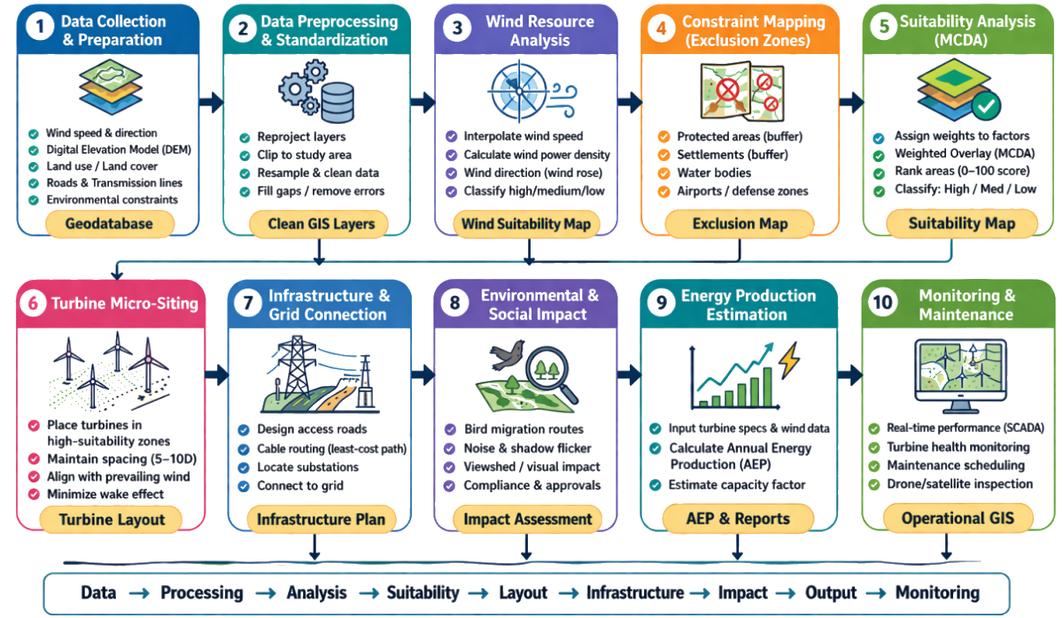
GIS data: Vector format vs Raster format
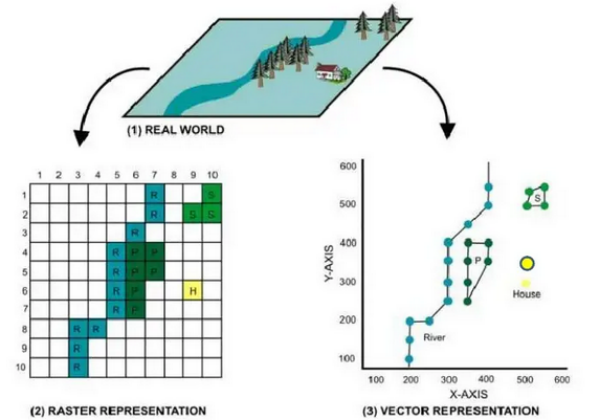
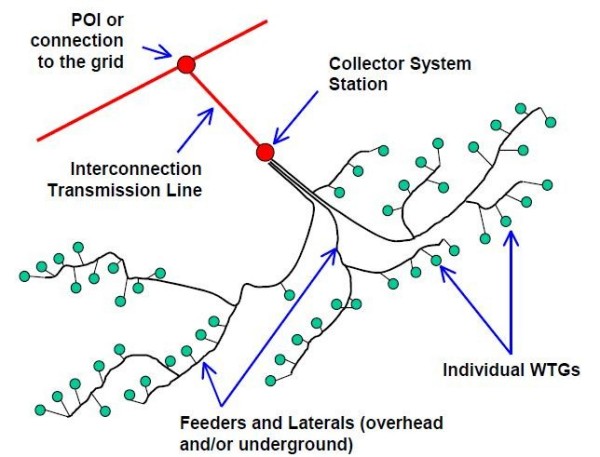
Wind Rose Diagram
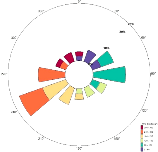

Interview questions related to wind-yield engineer
- How do you create a wind rose diagram?
- Name the inputs which most strongly affect AEP.
- What are P50, P75 and P90 and what are their use/importance?
- How do you respond to a situation where modeled AEP is consistently underestimates or overestimates the AEP?
- How do you use Geographical Information System data during site identification and feasibility studies?
- How do you handle sparse measurement data for complex terrain sites?
- What GIS checks are critical before finalizing micro-siting of turbines?
- Explain the role of MCP (Measure-Correlate-Predict) methods. Which techniques have you used?
- How do you handle missing or noisy wind data?
Mesoscale Meteorology
As per atmos.uw.edu/academic/mesoscale.html: "Mesoscale meteorology is the study of atmospheric phenomena with typical spatial scales between 10 and 1000 km. Examples of mesoscale phenomena include thunderstorms, gap winds, downslope windstorms, land-sea breezes, and squall lines. Many of the weather phenomena that most directly impact human activity occur on the mesoscale."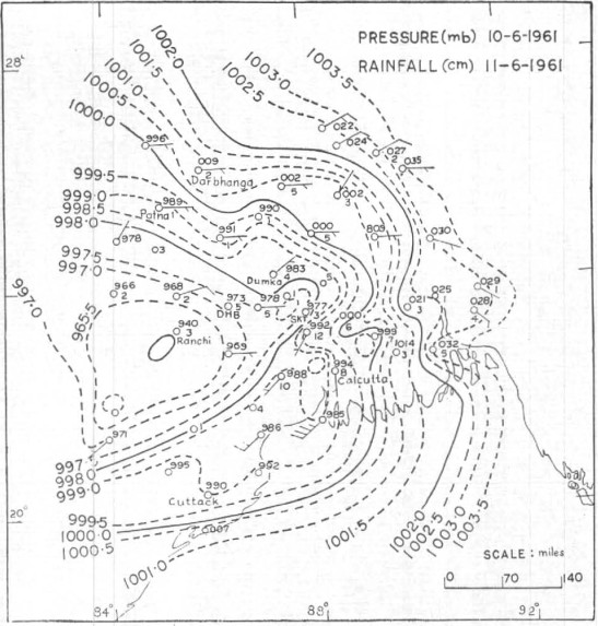
SCADA: Supervisory Control and Data Acquisition
This is a method or system to monitor, gather, and process data real-time by directly interacting with devices such as sensors, valves, pumps, motors... through human-machine interface (HMI) software. It record events into a log file. For example, the power producers or original equipment manufacturers (OEM) can monitor the performance of their turbines real time. The Programmable Logic Controllers (PLC) are hardware devices used for real-time control of individual machines or assets, operating at a smaller scale. SCADA systems include both software and hardware providing the visualization and analysis of data real-time.Fluid Pressure in Rotating Reference Frame
Bernoulli’s equation in the rotating frame where rotation is around z-axis: p(r, z) + ρgz + V(r) = p(r, z) + ρgz − ρω2r2. For a container open to atmosphere, gauge pressure at all points on the interface is zero i.e. p(r, z) = 0. Elevation of the free surface to the radial location: z = ω2r2/2/g.For a container rotating cylindrical about its axis: the shape of the free surface is a parabola and fluid inside the rotating cylinder forms a paraboloid of revolution, whose volume is one-half of the volume of the "circumscribing cylinder". To calculate angular velocity at which the liquid at the center reaches the bottom of the cylinder just as the liquid at the curved wall reaches the top of the cylinder: ωspill = (2gH)0.5/R.
Ball in rotating tube
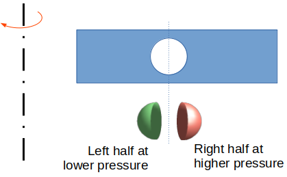
The centroid of a hemi-sphere is at 3R/8 from the base. Using this value, pressure on the left half of the ball = 1/2.ρF ω2(r-3R/8)2. The pressure on the right half of the ball = 1/2.ρF ω2(r+3R/8)2. Net force acting on the ball towards the axis of rotation = 1/2.ρF ω2(4.r.3R/8)2 × π*R2 where projected area = π*R2.
Net force due to fluid pressure towards axis of rotation, FF = 1/2.πR2.ρF ω2(r.3R/2) = 3/4πR3.ρF ω2r
Centrifugal force due to own mass of the ball, FB = 4/3.πR3.ρB ω2r
The position of the ball can be estimated using inequality FB ≤ FF. Will the ball get pushed towards inner radius for all densities of the ball? This method yielded incorrect conclusion as the pressure on the surface of spherical ball was assumed to be varying linearly with radius instead of parabolic variation as per formula p(r) = p(r = r0) + 1/2.ρFω2r2. The correct derivation of net fluid forces acting on the ball are given below: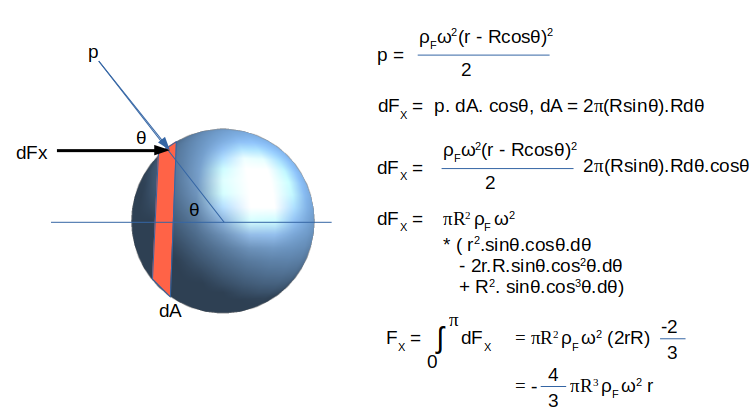
Root or Lobe Pump and Blowers
References
- ANSYS FLUENT User Manual
- Study of mesh deformation features of an open source CFD package and application to a gear pump simulation: Alejandro Roger Ull, ETSEIAT 2012
- NASA TM-73890: Gas Path Sealing in Turbine Engines
- Blade-Resolved, Single-Turbine Simulations Under Atmospheric Flow: by Michael Lawson et. al.
The content on CFDyna.com is being constantly refined and improvised with on-the-job experience, testing, and training. Examples might be simplified to improve insight into the physics and basic understanding. Linked pages, articles, references, and examples are constantly reviewed to reduce errors, but we cannot warrant full correctness of all content.
All Rights Reserved - CFDyna.com
Template by OS Templates