- CFD, Fluid Flow, FEA, Heat/Mass Transfer
Fluid Mechanics & Heat Transfer
Textbook Solutions: Fluid Mechanics, Heat & Mass Transfer, Aerodynamics
FM, HTX, MTX, AERO, COMBUSTION
This page is being continuously updated with complex (text-book type) problems in Fluid Mechanics, Heat Transfer, Aerodynamics, Mass Transfer, Combustion and Thermodynamics. The solutions to compressible flows including sub-sonic, sonic and supersonic flows inside a converging-diverging nozzle will be presented.
Table of Contents:
Buoyancy \-\ Plug Flow between Parallel Plates \-\ Flow through Pipe Branches forming Tee or Wye Network \-\ Equation of State: Soave-Redlick-Kwong Equation \-\ Half Filled Rotating Tube \+\ Thermal Network Example Calculations \=\ Steps to Create a Thermal Network Solver \=\ TNSolver Examples \=\ Fluid Network Solver \+\ Hardy-Cross Method Example \/\ Example: 3-Reservoirs System
Newton-Raphson Method \/\ Example Validation Cases \:\ Basic Fluid Network Solver \=\ Helper Functions to Develop the Solver in Java \=\ Fixed-flow and Pressure-jump Example: Python \:\ Fixed-flow and Pressure-jump Example: Java \+\ User Guide and Limitation of the Network Solver \@\ Sample Java Code based on Picard IterationsSummary of Hydrostatics
- For a plane surface immersed in a liquid in any orientation, the total normal pressure over the surface is P = A * ρ * g * h where h is the vertical depth of the centre of the gravity of the surface from free surface of the liquid, A is area of the surface.
- A plane surface immersed in a liquid is acted upon by a system of parallel forces which can be reduced to act on a single point of the surface known as centre of pressure.
- A curved surface immersed in a liquid is not acted upon a "system of parallel forces" and hence in general they cannot be reduced to a single force.
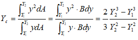
Centre of pressure of vertical rectangular plate
This is a very useful case which has frequent engineering applications.
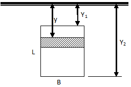
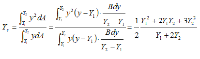
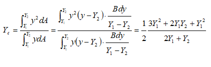
Similarly, for a triangular plate with base horizontal and at depth of Y2 and vertex up at depth of Y1, the centre of pressure is given by:
Centre of pressure of vertical circular plate
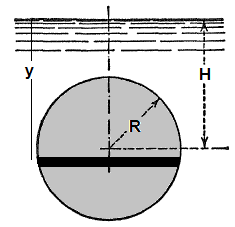
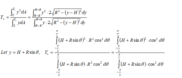
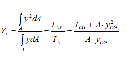
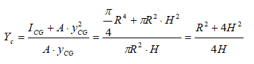
Even though the complicated definite integration is possible analytically, this is the time the introduce a simple method based on properties of sections. Note that the numerator of expression for centre of pressure is the "Second Moment of Inertia" or simply the Moment of Inertia about a "chosen axis" - typically the free surface of the liquid. The denominator is the "Moment of Area" about the same axis as chosen above - also known as "Statical Moment". Thus:
- If the area has axis of symmetry about the vertical axis, the centre of pressure will fall on it.
- Conversely, the centre of pressure will fall on the medial line, the vertical axis passing through the centre of gravity on the horizontal axis.
- The position of the centre of pressure is always below the centre of gravity of a surface.
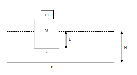
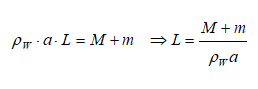
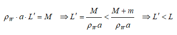
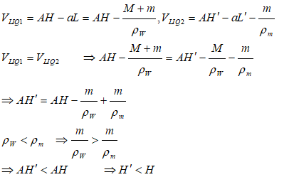
Buoyancy - Example Problem
A metallic block is floating along with a wooden block as shown in the figure below. If this metallic block falls into the tank, calculate the new depth of floatation and height of water level in the tank.
Analogy Between Fluid Flow, HTX and MTX
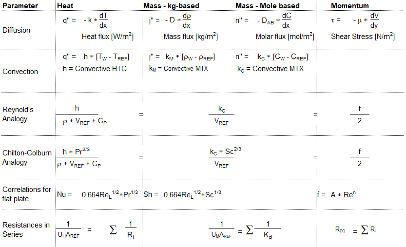
The method of relating two phenomena with some come feature is a powerful tool to both understand and remember the concepts. Following table summarizes key parameters which are analogous in the field of fluid flow (momentum transfer), heat transfer and mass transfer.
1D Heat Transfer with Convective Boundaries and Heat Generation
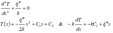
The designs of heat exchangers are the most predominant application of conductive heat transfer with such boundary conditions. The temperature profile in walls of a water-cooled internal combustion engine is also subject to this combination of boundary conditions though heat generation is not present in this application. Some applications can be current carrying conductor cooled by convection on both inner and outer diameters, nuclear fission in a annular cross-section cooled by convection on both the inner and outer radii. The governing equation and general solution of the differential equation is given by
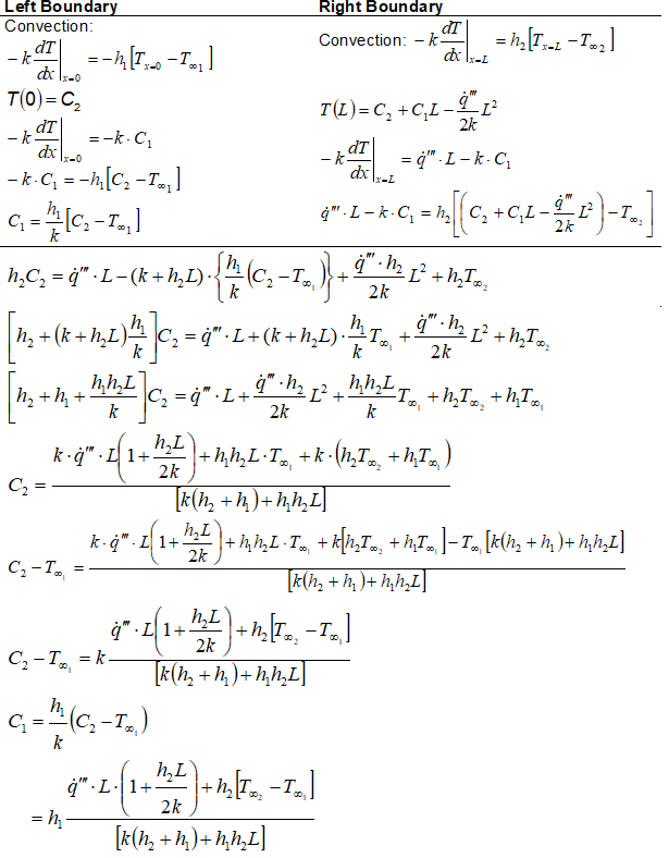
Heat flow is assumed positive from left to right. Hence, the convective heat transfer on left face is negative if ambient temperature is < wall temperature on the left face!
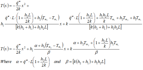
Finally, the temperature distribution function is expressed as:
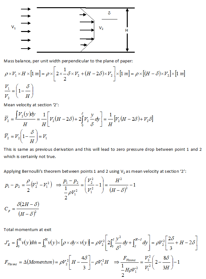
Plug Flow between Parallel Plates
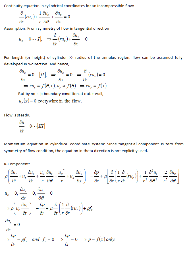
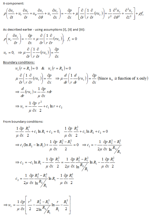
Flow in an Annular Passage
Flow through Pipe Branches forming Tee or Wye Network
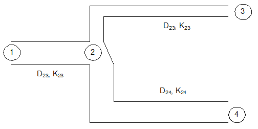
Note velocities in pipe branches 1-2, 2-3 and 3-4 are not known in advance and hence the loss coefficients KMN cannot be adjusted to same velocity. Note that the junction losses at node 2 can be incorporated either in K12 or in K23 and K24. It is more convenient to club the node loss in K12 as appropriate assignment into K23 and K24 will involve extra calculations.
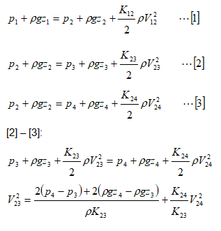
Denoting the pressures in terms of head of water column:
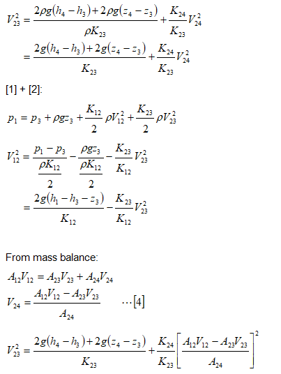
Simplifying further:
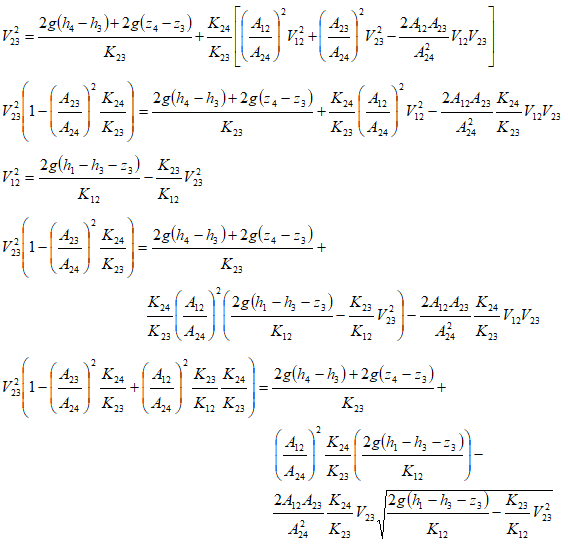
This is a non-linear equation in V23 and needs to be solved using trial-and-error or iterative approaches. Microsoft Excel Goal Seek utility can be used to solve this equation as well. A good initial guess would be required.
A more compact approach in terms of fluid resistances can be used as demonstrated below.
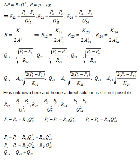
Thus, we have 3 equations and 3 unknowns – but they are still non-linear and needs to be solved using iterative method.
Force on a curved pipe with varying cross-section
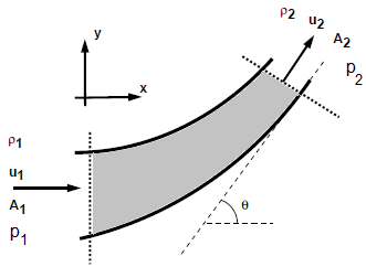
A reducing bend having diameters D upstream and d downstream, has water flowing through it at the rate of m [kg/s] under a pressure of p1 bar. Neglecting any loss is head for friction calculate, the horizontal and vertical components of force exerted by the water on the bend.
Newton's Law of Motion applied to Fluid Elements:
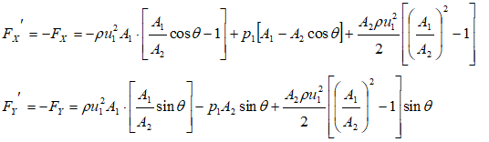
F = m [u2 - u1]Newton's Third Law Applied to Pipe:
This is the force acting on the fluid and only means to apply the force on the fluid is the walls of the pipe. Hence, from Newton’s third law, and equation and opposite force will act on the pipe.
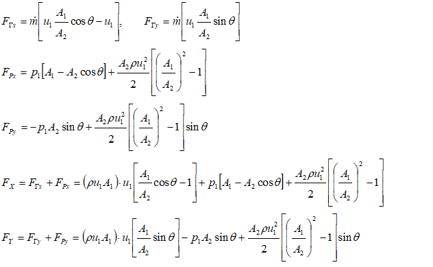
ΔΓX = m * [u2X - u1X] = FΓX. Thus: FΓX = m * [u2 cos(θ) - u1]ΔΓY = m * [u2Y - u1Y] = FΓY. Hence, FΓY = m * [u2 sin(θ) - 0] = m * u2 sin(θ)
Force on fluid element due to pressure at boundaries
FpX = p1A1 - p2A2cos(θ)FpY = 0 - p2A2sin(θ)
Use Bernoulli’s equation to find p2 in terms of other known parameters:
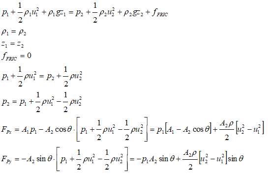
If pipe is straight
θ = 0 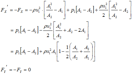
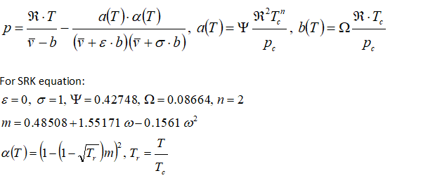
Equation of State: Soave-Redlick-Kwong Equation
or gases at very high pressure and those in liquid state such as Liquified Petrolium Gas (LPG), the accuracy of ideal gas equation falls sharply. Many improvizations have been made and SRK equation is one such method. The approach is demonstrated using following sample problem:
A gas cylinder with a volume of 5.0 m3 contains 44 kg of carbon dioxide at T = 273 K. estimate the gas pressure in [atm] using the SRK equation of state. Critical properties of CO2 and Pitzer acentric factor are: Tc = 304.2 K, pc = 72.9 atm, and ω = 0.225.
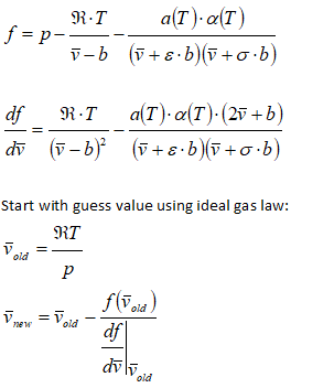
General cubic equation of state is given by following equation
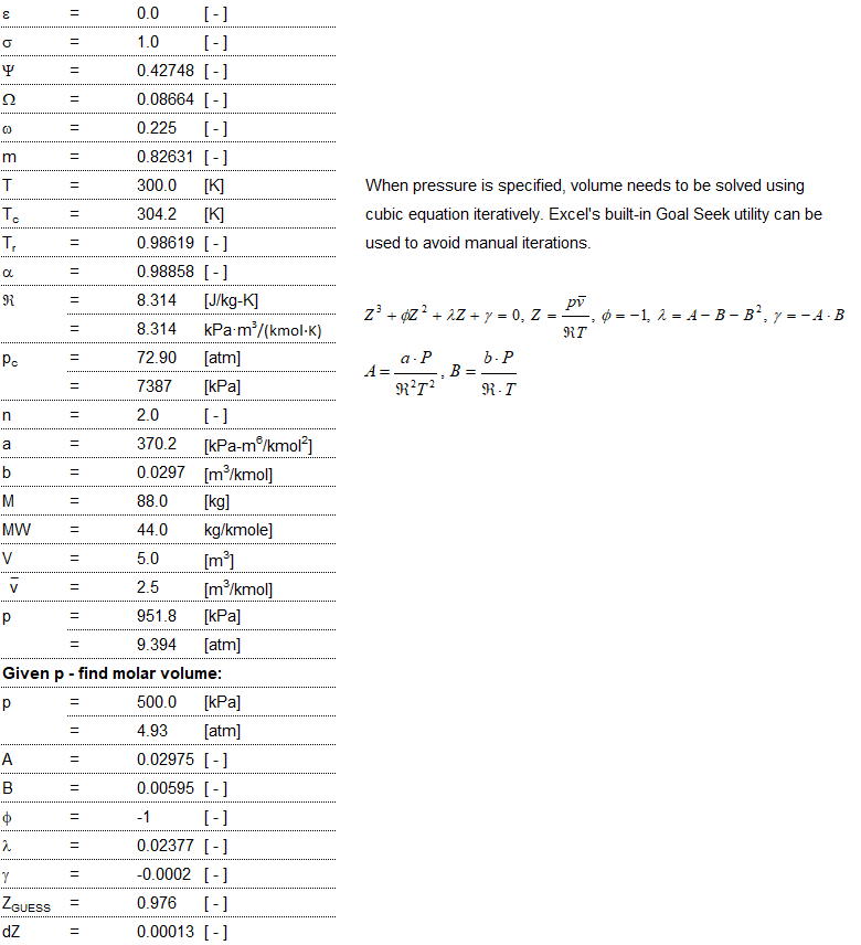
Alternatively, the equation can be solved using Newton's method as described below.
Hydrostatics in Rotating Reference Frame
The equation of equilibrium of fluid particles rotating about any fixed axis (say Z-axis) and acted about forces in 3 directions is given by:dp = ρ . {FX dx + FY dy + FZ dz + ω2(xdx + ydy)} where FX is the force per unit volume is X-direction. Alternatively, dp = ρ . {FX dx + FY dy + FZ dz + ω2rdr}. Any point where liquid separates is the location where pressure vanishes i.e. p = 0. Latus rectum of free surface = 2g/ω2.

Half Filled Rotating Tube: A circular tube is half full of liquid and is made to revolve around a vertical tangent line with angular velocity ω. If radius of the tube is R, calculate the angle between horizontal and diameter passing through the free surface of the liquid.
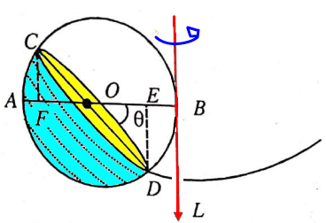
The tube is rotating about red line and the liquid level is shown by yellow zone. Point 'D' is the lower most point of free surface, θ is the angle which needs to be calculated.
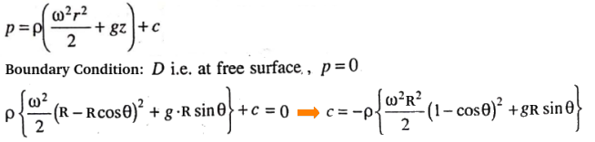
The pressure at any location is given by: dp = ρ (ω2r.dr + gdz) where r is the distance of the point from the axis of rotation and z is the distance of the point from the origin. The point 'D' is rotating at radius r = R(1-cosθ), z = R.sinθ and is at p = 0. Another known point 'C' is at pressure zero, r = R(1+cosθ), z = -Rsinθ. Note that +z is along the downward direction (this is only a convention).
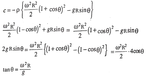
Liquid filled in rotating conical pot: A conical pot of height H and vertical (full cone) angle θ contains liquid k-times (x < 1) the volume of full cone. Find out the minimum angular velocity at which shall prevent liquid overflowing the cone.
Thus; z = (1-k).2H/3 ... [1] Also, from paraboloid of revolution (latus rectum): 2g/ω2 = R2/z ⇒ z = ω2.R2/2/g ... [2]
To prevent overflow: z ≤ (1-k).2H/3From equations [1] and [2], ω2.R2/2/g ≤ (1-k).2H/3 ⇒ ω ≤ [4g/3.(1-k).H/R2]1/2
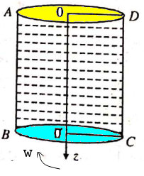
R = H . tan(α) ⇒ ω ≤ [4g/3H.(1-k)]1/2.cot(α), thus if k = 0.5, ω ≤ [2g/3H]1/2.cot(α)A closed circular cylinder is just filled with water and rotates about a vertical. Find the ratio of total thrust on the bottom to that on the top when the angular velocity is ω, H is the height and R the radius of the cylinder.
Fluid Pressure in Rotating Reference Frame
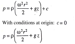
Bernoulli’s equation in the rotating frame where rotation is around z-axis: p(r, z) + ρgz + V(r) = p(r, z) + ρgz − ρω2r2. For a container open to atmosphere, gauge pressure at all points on the interface is zero i.e. p(r, z) = 0. Elevation of the free surface to the radial location: z = ω2r2/2/g.For a container rotating cylindrical about its axis: the shape of the free surface is a parabola and fluid inside the rotating cylinder forms a paraboloid of revolution, whose volume is one-half of the volume of the "circumscribing cylinder". To calculate angular velocity at which the liquid at the center reaches the bottom of the cylinder just as the liquid at the curved wall reaches the top of the cylinder: ωspill = (2gH)0.5/R.
Ball in rotating tube
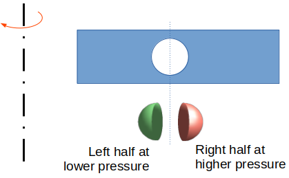
The centroid of a hemi-sphere is at 3R/8 from the base. Using this value, pressure on the left half of the ball = 1/2.ρF ω2(r-3R/8)2. The pressure on the right half of the ball = 1/2.ρF ω2(r+3R/8)2. Net force acting on the ball towards the axis of rotation = 1/2.ρF ω2(4.r.3R/8)2 × π*R2 where projected area = π*R2.
Net force due to fluid pressure towards axis of rotation, FF = 1/2.πR2.ρF ω2(r.3R/2) = 3/4πR3.ρF ω2r
Centrifugal force due to own mass of the ball, FB = 4/3.πR3.ρB ω2r
The position of the ball can be estimated using inequality FB ≤ FF. Will the ball get pushed towards inner radius for all densities of the ball? This method yeilded incorrect conclusion as the pressure on the surface of spherical ball was assumed to be varying linearly with radius instead of parabolic variation as per formula p(r) = p(r = r0) + 1/2.ρFω2r2. The correct derivation of net fluid forces acting on the ball are given below: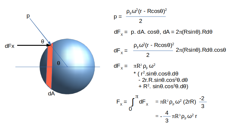
A circular cylinder of radius 'a' whose axis is vertical, is filled to depth h with homogeneous liquid of density ρ. Find the pressure as function of radial and vertical positions. Also, find the forces acting on the top lid if closed.

dp = ρ{-g.dz + ω2rdr} -> p = ρ{-g.z + 1/2.ω2r2} + C
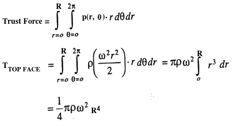
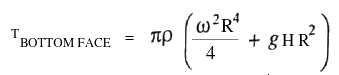
Applying boundary condition at centre of top surface, p = 0 at r = 0 and z = h, C = ρgh. Thus, p = ρ{-g.z + 1/2.ω2r2} + ρgh and pressure at any point on top lid can be found by z = h. The thrust on the top lid is:
A hollow cone nearly filled with water, rotates uniformly about its axis which is vertical, the vertex being uppermost. Find the total thrust on the base of the cone. 'a' is the radius of the base and 2α the vertical angle of the cone.

p = ρ{-g.z + 1/2.ω2r2} + ρgh
At the base of the cone, z = 0. Thus, p(z=0) = ρ{1/2.ω2r2} + ρgh
Practice Questions:
- A hollow sphere of radius 'R' is half-filled with liquid and is rotating at angular velocity ω about its vertical diameter. Find out the value of ω at which the lowest point of the sphere is just exposed. Answer: [2g/R]1/2.[2-41/3]-1/2. Hint: volume of water remains constant.
- A narrow annular horizontal tube of radius R containing liquid is filled to half of its circumference and is rotating about the vertical diameter with angular velocity ω. Calculate the value of angular velocity at which liquid will just separate. Answer: [2g/R]1/2. Hint: pressure will become zero at lowest point when liquid separates.
- A vertical inverted conical vessel (base at the top) of height 'h' and cone angle 2θ is half-filled with a liquid oil. Find out the maximum angular velocity ω at which the oil shall not overflow. Answer: [2g/3h]1/2.cot(θ) Hint: use latus rectum as defined earlier.
Steps to Create a Thermal Network Solver
Step-0: Define problem set-up: Steady or Transient, Initial Temperature, Total Run Time, Time Step Solution, Time Step Data Save.
Step-1: Define input table for the network. For Steady state cases, Cp and Mass shall be neglected.
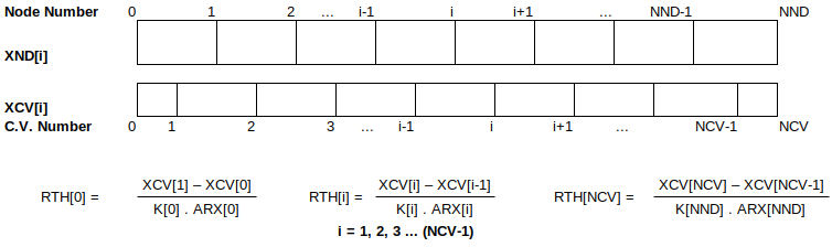
Note that: NND = number of nodes, NCV = Number of control volumes = NND+1, XND[0] = XCV[0] = 0, XCV[i] = (XND[i+1] + XND[i] ) / 2 for i = 1 to NND-1, XCV[NCV] = XND[NND]. LCV[0] = XND[1]/2, LCV[i] = XCV[i] - XCV[i-1], LCV[NCV] = 0.5 x (XND[NND] - XND[NND-1])
| Node | T | ARX | Cp | Mass | Connected Nodes | ||
| [No.] | [C] | [m2] | [J/kg-K] | [kg] | [No.] | ||
| 1 | 0 | 0.01 | 2700 | 0.10 | 2 | 3 | - |
| 2 | 0 | 0.01 | 1200 | 0.05 | 1 | 3 | 4 |
| 3 | 40 | 0.01 | 1200 | 0.02 | 1 | 5 | 2 |
| 4 | 0 | 0.01 | 500 | 0.01 | 3 | - | - |
| ... | ... | ... | ... | ... | ... | ... | ... |
Step-2: Define resistance table. All information can be supplied as CSV file in following order (use negative number for boundary nodes). Here, Tref can be used to specified reference temperature for nodes with HTC boundary conditions as well as nodes with known or fixed temperatures. Value of 0 for Temperature or Tref indicate unknown or optional. There are some limitations to define the nodes such as a node must be placed where there is step change of cross-section. The node numbering must start with 1 and increase sequentially without any gap.
           [3]      [6]
            |        |
            |        |
[1]--------[2]------[5]-------[8]-------[9]-------[10]
            |        |
            |        |
           [4]      [7]
R_ID, s_node, e_node, xLen,  xAr,      k,     Cp,    Den
R01,  1,      2,      0.050, 0.0005, 200.0, 500.0, 2700.0
R02,  2,      3,      0.025, 0.0005, 200.0, 500.0, 2700.0
R03,  2,      4,      0.025, 0.0005, 200.0, 500.0, 2700.0
R04,  2,      5,      0.125, 0.0005, 200.0, 500.0, 2700.0
R05,  5,      6,      0.025, 0.0005, 200.0, 500.0, 2700.0
R06,  5,      7,      0.025, 0.0005, 200.0, 500.0, 2700.0
R07,  5,      8,      0.025, 0.0005, 200.0, 500.0, 2700.0
R08,  8,      9,      0.025, 0.0005, 200.0, 500.0, 2700.0
R09,  9,     10,      0.025, 0.0005, 200.0, 500.0, 2700.0
Use one line function to calculation thermal resistance and thermal inertia (capacitance) - lambda functions can also be used.
def calcThermalRes(xL, xA, xk):
  return xL/xA/xk
def calcThermalIntertia(xL, xA, xDen, xCp):
  return xDen * (xL * xA) * xCp
Inputs for nodes, note that symbol Tref is used both for specified node temperature and reference temperature in case of convective boundary conditions.
NN stands for Node Number
-------------------------
NN,   Qdot,  HTC,    Tref
 1,    0,     0,     288
 2,   50,     0,     0
 3,   50,     0,     0
 4,   50,     0,     0
 5,    0,     0,     0
 6,    0,     0,     323
 7,    0,    10,     298
 8,    0,    10,     298
 9,    0,     0,     0
10,    0,     0,     373
import csv
def csvToColumnLists(csv_file):
  '''
  Reads a CSV file and returns a dictionary where keys are column headers
  and values are lists containing the data for each column. First non empty
  row is assumed to be header containing strings without spaces. Header names
  are case-sensitive.
  '''
  column_data = {}
  with open(csv_file, 'r', newline='') as file_csv:
    reader = csv.reader(file_csv)
    headers = next(reader)
    headers = [header.strip() for header in headers]
    # Initialize empty list for each header and append data
    for header in headers:
      column_data[header] = []
    for row in reader:
      for i, value in enumerate(row):
        column_data[headers[i]].append(value.strip())
  return column_data
#
data_r = csvToColumnLists('thermal_r.csv')
node_col_1 = data_r['s_node']
node_col_2 = data_r['e_node']
node_col_1 = [int(NN) for NN in node_col_1]
node_col_2 = [int(NN) for NN in node_col_2]
xL = data_r['xLen']

# Find names of nodes as union of sets from column 2 and 3
NNU = list(set(node_col_1) | (set(node_col_2)))
NNU = [int(N) for N in NNU]
NNU.sort()

NNL = node_col_1 + node_col_2
max_n = int(max(set(NNL), key=NNL.count))
NNR = len(data_r['R_ID'])
NMAT = [[0] * max_n] * NNR
Create thermal resistance 2D array
def createRTH(xLen, xAr, xk, node_i, node_j):
  '''
  Create thermal resistance as 2D matrix, the size of matrix is 1 greater than
  the maximum node number in the network. Note that node numbering starts from
  1 and increase sequentially without any gap or step.
  '''
  NTH = int(max(max(node_i), max(node_j)))
  NR = len(node_i)
  RTH = []
  for _ in range(NTH):
    row = [0] * NTH
    RTH.append(row)

  for i in range(0, NR):
    m = int(node_i[i]) - 1
    n = int(node_j[i]) - 1
    RTH[m][n] = float(xLen[i]) / float(xAr[i]) / float(xk[i])
    RTH[n][m] = RTH[m][n]
  return RTH
Step-3: Define governing equations using energy balance at each nodes with unknown temperatures and nodes with known temperatures.
For node-1 above: (T1 - T2)/R12 + (T1 - T3)/R13 = Qdot1
or
A1 T1 + B12T2 + B13T3 = Qdot1 where the second values in the subscripts correspond to entry under "Connected Nodes".
For node-2 above: (T2 - T1)/R12 + (T2 - T3)/R23 + (T2 - T4)/R24 = Qdot2
or
A2 T2 + B21T1 + B23T3 + B24T4 = Qdot2 where the second values in the subscripts correpond to entry under "Connected Nodes".
Step-4: Convert the individual equations into equivalent index notation (subscripts converted into indices of arrays).
Step-5: Define variables and arrays. NND = number of nodes, 1D arrays: XND[NND], XCV[NCV] Qdot[NND], Cp[NND], mass[NND], cond[NND], XAR[NND], LCV[NND]. 2D arrays: coeff_a[NND, NND], coeff_b[NND, NND], coeff_c[NND, NND], th_res[NND, 10], con_nodes(NND, 10). Each node is assumed to be connected to maximum 10 nodes.
Write functions to approximate differential equations
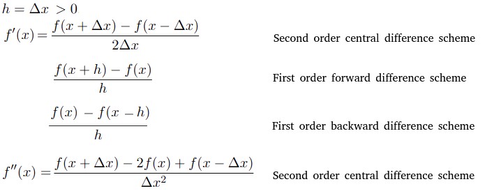
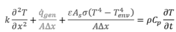
For steady state 1D heat conduction with volumetric heat generation and convective heat loss:
Another example from web:
Training Project: Development of thermal network model and validation of results with 3D CFD simulations using ANSYS Fluent or OpenFOAM is a good internship project. This will impart not only programming skills but also help the engineer gain insight into heat transfer and matrix algebra.
Thermal Network Example Hand Calculations
Assume all heat flowing into a node is positive and all nodes around it are at higher temperatures. Final result will amend this assumption to correct values.q'[100W]----->[1]-------[2]--------[3]== T [300 K]
L: 0.10 [m]
A: 5E-4 [m2]
k: 50.0 [W/m-K]
Thermal Resistance: R12 = R23 = k/L/A = 4.0 [K/W]
Node-1:
 1/R12 * [T2 - T1]                     = q'
Node-2:
 1/R12 * [T2 - T1] + 1/R23 * [T2 - T3] = 0
-1/R12 * [T1] + [1/R12 + 1/R23] * [T2] = T3/R23
-1/R12 * [T1] + [1/R12 + 1/R23] * [T2] = T3/R23
Matrix to solve
-1/R12 * [T1] + 1/R12           * [T2] = q'
-1/R12 * [T1] + [1/R12 + 1/R23] * [T2] = T3/R23
Some other configurations that can serve as validation for any thermal network solver are:
q'[100 W]----->[1]-------[2]--------[3]== T [300 K]
                          |
                          |
                         [4]
                      q' [50 W]


                      HTC: 20 [W/m2-K], TREF=300 [K]
                         [5]
                          |
                          |
q'[100 W]----->[1]-------[2]--------[3]== T [300 K]
                          |
                          |
                         [4]
                       q' [50 W]
Generic node in a thermal network:
                [s]   [r]   [p]
              .'  \    |   /
             '     \   |  /
            '        *[n]'--------  [m]
            '          |
             ` ,       |
                 ` - =[u]
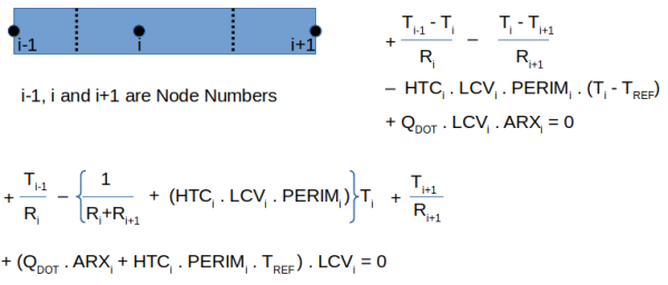
Assuming heat 'q' [W] is generated at node 'n' and all surrounding nodes are at lower temperatures:
[Tn - Tm]/RTH[n,m] + [Tn - Tp]/RTH[n,p] + ... + [Tn - Tu]/RTH[n,u] + h.A.[Tn - Tref] = q
{1/RTH[n,m] + 1/RTH[n,p] + ... + 1/RTH[n,u] + h.A}*Tn - 1/RTH[n,m]*Tm - ... - 1/RTH[n,u]*Tu = q + h.A.TrefΣj(1/RTH[n, j]) . Tn - {Σj[1/RTH[n,j] . Tj} = q + h.A.Tref ... ... ...[1]
In terms of thermal conductances:Σj(CTH[n, j]) . Tn - {Σj[CTH[n,j] . Tj} = q + h.A.Tref ... ... ...[2]
Next step: create thermal resistance 2d array. RTH[j,k] are calculated earlier and known for all j and k - sparse symmetric matrix, RTH[j, k] = RTH[k, j] and diagonal entries = 0. Note that thermal resistances by definition are always positive, a negative value is used to indicate direction of heat transfer.
Thermal Resistance Array:
       1 |     2 |     3 |     4 |     5 |     6 |     7 |     8 |     9 |    10 |
 --------|-------|-------|-------|-------|-------|-------|-------|-------|-------|
 1     0 |  0.50 |     0 |     0 |     0 |     0 |     0 |     0 |     0 |     0 |
 2  0.50 |     0 |  0.25 |  0.25 |  1.25 |     0 |     0 |     0 |     0 |     0 |
 3     0 |  0.25 |     0 |     0 |     0 |     0 |     0 |     0 |     0 |     0 |
 4     0 |  0.25 |     0 |     0 |     0 |     0 |     0 |     0 |     0 |     0 |
 5     0 |  1.25 |     0 |     0 |     0 |  0.25 |  0.25 |  0.25 |     0 |     0 |
 6     0 |     0 |     0 |     0 |  0.25 |     0 |     0 |     0 |     0 |     0 |
 7     0 |     0 |     0 |     0 |  0.25 |     0 |     0 |     0 |     0 |     0 |
 8     0 |     0 |     0 |     0 |  0.25 |     0 |     0 |     0 |  0.25 |     0 |
 9     0 |     0 |     0 |     0 |     0 |     0 |     0 |  0.25 |     0 |  0.25 |
10     0 |     0 |     0 |     0 |     0 |     0 |     0 |     0 |  0.25 |     0 |
The thermal conductance matrix is:
       1 |     2 |     3 |     4 |     5 |     6 |     7 |     8 |     9 |    10 |
 --------|-------|-------|-------|-------|-------|-------|-------|-------|-------|
 1     0 |   2.0 |     0 |     0 |     0 |     0 |     0 |     0 |     0 |     0 |
 2   2.0 |     0 |   4.0 |   4.0 |   0.8 |     0 |     0 |     0 |     0 |     0 |
 3     0 |   4.0 |     0 |     0 |     0 |     0 |     0 |     0 |     0 |     0 |
 4     0 |   4.0 |     0 |     0 |     0 |     0 |     0 |     0 |     0 |     0 |
 5     0 |   0.8 |     0 |     0 |     0 |   4.0 |   4.0 |   4.0 |     0 |     0 |
 6     0 |     0 |     0 |     0 |   4.0 |     0 |     0 |     0 |     0 |     0 |
 7     0 |     0 |     0 |     0 |   4.0 |     0 |     0 |     0 |     0 |     0 |
 8     0 |     0 |     0 |     0 |   4.0 |     0 |     0 |     0 |   4.0 |     0 |
 9     0 |     0 |     0 |     0 |     0 |     0 |     0 |   4.0 |     0 |   4.0 |
10     0 |     0 |     0 |     0 |     0 |     0 |     0 |     0 |   4.0 |     0 |
Next step: find out nodes with known temperature.
data_n = csvToColumnLists('thermal_n.csv')
node_nnum = data_n['NN']
node_nnum = [int(NN) for NN in node_nnum]
node_hgen = data_n['Qdot']
node_hgen = [float(x) for x in node_hgen]
node_htc  = data_n['HTC']
node_htc  = [float(x) for x in node_htc]
node_Tref = data_n['Tref']
node_Tref = [float(x) for x in node_Tref]
node_known_T = [
  item_1 for item_1, item_2, item_3 in zip(node_nnum, node_htc, node_Tref)
  if item_2 == 0 and item_3 != 0
]
Next step: create node connectivity matrix. The matrix of each node and connected nodes (the indices for summation over index i in equation above) except for those with known/specified temperatures, can be estimated as follows.
Node connectivity array:
    2 |     1 |     3 |     4 |     5 |
    3 |     2 |     0 |     0 |     0 |
    4 |     2 |     0 |     0 |     0 |
    5 |     2 |     6 |     7 |     8 |
    7 |     5 |     0 |     0 |     0 |
    8 |     5 |     9 |     0 |     0 |
    9 |     8 |    10 |     0 |     0 |

           [3]      [6]
            |        |
            |        |
[1]--------[2]------[5]-------[8]-------[9]-------[10]
            |        |
            |        |
           [4]      [7]
Using Σj(CTH[n, j]) . Tn - {Σj[CTH[n,j] . Tj} = q + h.A.Tref ... ... ...[2]
Node-2: Generic internal Node connected with more than 1 node.
(C[2, 1] + C[2, 3] + C[2, 4] + C[2, 5]) * T[2]
                              - C[2, 3] * T[3]
                              - C[2, 4] * T[4]
                              - C[2, 5] * T[5]
                              = C[2, 1] * T[1] + q[2] + h[2] * A[2] * (T[2] - Tref[2])

A[0, 1]*T[2] + A[0, 2]*T[3] + A[0, 3]*T[4] + A[0, 4]*T[5] = B[1]
Node-3: Boundary Internal Node connected with 1 node but also to a virtual node due to HTC boundary conditions.
C[3, 2] * (T[3] - T[2]) = q[3] + h[3] * A[3] * (T[3] - Tref[3])

A[1, 0]*T[2] + A[1, 2]*T[3]                               = B[2]
Node-4: convection node
C[4, 2] * (T[4] - T[2]) = q[4] + h[4] * A[4] * (T[4] - Tref[4])

A[2, 0]*T[2]                + A[2, 3]*T[4]                = B[3]
Node-5:
(C[5, 2] + C[5, 6] + C[5, 7] + C[5, 8]) * T[5]
                              - C[2, 5] * T[2]
                              - C[7, 5] * T[7]
                              - C[8, 5] * T[8]
                              = C[7, 5] * T[7] + q[5] + h[5] * A[5] * (T[5] - Tref[5])
A[3, 0]*T[2] +                             + A[3, 4]*T[5] + A[3, 6]*T[7] + A[3, 7]*T[8] = B[4]
Next step: generate coefficient matrix as per equation [1] above. Compute the number of nodes with unknown temperature from node connectivity matrix. The coefficient matrix A[i, j] would be of size N x N where N is number of rows in node connectivity array defined above. phi_T = [row[0] for row in node_con_array] to get first column which contains node numbers for which temperature needs to be calculated.
Note:
- Arrays start with index zero but the lowest item in node connectivity matrix may be any number ≥ 1
- Coefficient matrix cannot have any element on diagonal row = zero
- The thermal resistance values are linked to node numbers and stored as rows and columns defined by connected nodes
- Thermal resistance matrix contains 0 values and hence a check is required to calculate the inverse of thermal resistances
Get first column of each row as center node: row_i = node_con_mat[i]; n_num = row_i[0]
Inner Loop Loops over second item onwards on each row
Calculate diagonal item of coefficient matrix A[i, i]
The initial coefficient matrix is as follows. Note that the rows and columns corresponding to nodes with specified temperature are all not required for final matrix inversion (solution of temperature values). Also, the coefficient matrix need not be symmetric.10.8 | -4.0 | -4.0 | -0.8 | 0.0 | 0.0 | 0.0 | -4.0 | 4.0 | 0.0 | 0.0 | 0.0 | 0.0 | 0.0 | -4.0 | 0.0 | 4.0 | 0.0 | 0.0 | 0.0 | 0.0 | -0.8 | 0.0 | 0.0 | 12.8 | -4.0 | -4.0 | 0.0 | 0.0 | 0.0 | 0.0 | -4.0 | 3.995 | 0.0 | 0.0 | 0.0 | 0.0 | 0.0 | -4.0 | 0.0 | 7.995 | -4.0 | 0.0 | 0.0 | 0.0 | 0.0 | 0.0 | -4.0 | 8.0 |
Computed value of {b} excluding for those with known T:
{b} = [626.0, 50.0, 50.0, 1292.0, 1.49, 1.49, 1492.0]Computed temperatures in [K]: for nodes in first column of node connectivity matrix above. Validation of result with hand calculation is in progress though values are very close to results produced by TNSolver (without HTC boundary conditions).
288.0
356.2
368.7
368.7
339.1
323.0
339.9
350.9
362.0
373.0
The results match with TNSolver values when convection is removed from nodes. Further enhancements planned for this code are:
- Give option to provide default length, cross-section area, material (thermal conductivity) for all resistors
- Let user chose positive integers for numbering nodes and not enforcing start from 1 without any gap
- Check correctness of inputs such as missing values, string instead of numbers...
- Add radiative heat transfer from resistors
- Add radiative heat transfer from nodes
- Add convection from resistors
- Add transient calculations
- Allow comments
- Single input file
The code can also be used to solve electrical networks where thermal conductivity 'k' needs to be replaced by electrical conductivity 'σ'. RTH = L/k/A, REL = ρ.L/A = L/σ/A where electrical conductivity σ = 1/ρ, ρ = electrical resistivity.
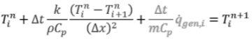
The example demonstrated above is linear and explicit where all coefficients and constants are independent of field variable 'T'. In cases where thermal conductivity is function of temperature or heat generation rate is function of temperature or cases like radiation where heat transfer rate is not a linear function of temperature [\(Q=\epsilon A\sigma (T^{4}-T_{∞}^{4})\)], the simple matrix inversion methods like y = np.linalg.solve(A, b) does not work. \[h_{rad}=\frac{\epsilon \sigma (T_{i}^{4}-T_{∞}^{4})}{(T_{i}-T_{∞})}\] which can be simplified (still non-linear) to \(h_{rad}=\epsilon \sigma (T_{i}+T_{∞})(T_{i}^{2}+T_{∞}^{2})\) The method above assumes that the ambient behaves like a black body. In case of radiative heat exchange between two non-black (grey) bodies and reflections of radiation are not taken into account: \[Q_{ij}^{RAD} = ε_i ε_j\cdot A_i F_{ij} (T_{i}^{4}-T_{j}^{4})\] When reflection of radiations are taken into account, some of the radiation coming from surface i gets reflected by surface j. A part of this reflected energy shall end up on other surfaces, which in their turn (if grey) shall reflect some fraction of the incident radiation. Radiative heat exchange between grey bodies is calculated using two different methods: Gebhart method and the Oppenheim method (Net Radiant Method).An iterative method like Jacobi or Gauss-Seidel iteration is required. The coefficient matrix A should ideally be diagonally dominant for guaranteed convergence. In Jacobi iteration, the value of each \(x_{i}\) at the new iteration is computed using the formula:
$$x_{i}^{(k+1)}=\frac{b_{i}-\sum \limits _{j\ne i}a_{ij}x_{j}^{(k)}}{a_{ii}}$$def Jacobi(A, b, x_0, max_iter=100, tolerance=1.0e-6):
'''
x_0: Initial guess for the solution, numpy array
tolerance: Convergence criteria
max_iter: Maximum number of iterations to perform
Returns: the approximate solution [vector].
'''
# Initialize the solution vector
x = x_0.copy()
n = len(b)
for k in range(max_iter):
x_new = x.copy()
for i in range(n):
# Calculate the sum of row elements, excluding diagonal value
sum_row = 0
for j in range(n):
if i != j:
sum_row = sum_row + A[i, j] * x[j]
x_new[i] = (b[i] - sum_row) / A[i, i]
# Check for convergence, np.inf = Maximum absolute value
L2NORM_new = np.linalg.norm(x_new - x, ord=np.inf)
L2NORM_old = np.linalg.norm(x_new, ord=np.inf)
if (L2NORM_new / L2NORM_old) <= tolerance:
print(f"Solution converged after {k+1} iterations.")
return x_new
x = x_new
print(f"Converge could not be achieved within {max_iter} iterations.")
return x
Gauss-Seidel Method: The convergence is guaranteed if the matrix A is strictly diagonally dominant [magnitude of diagonal entry ≥ sum of the magnitudes of non-diagonal entries for each row] or symmetric positive definite [square matrix that is equal to its transpose]. The Gauss-Seidel method often converges faster than the Jacobi method by using updated values within the same iteration.
def GaussSeidel(A, b, x_0, max_iter=100, tolerance=1.0e-6, ):
  A = np.array(A, dtype=float)
  b = np.array(b, dtype=float)
  x = np.array(x_0, dtype=float)
  n = len(b)
  for iter in range(max_iter):
    x_old = np.copy(x)
    for i in range(n):
      sum_ax = np.dot(A[i, :i], x[:i]) + np.dot(A[i, i+1:], x_old[i+1:])
      x[i] = (b[i] - sum_ax) / A[i, i]
    if np.linalg.norm(x - x_old) < tolerance:
      print(f"Convergence achieved after {iter + 1} iterations.")
      return x
  print(f"Run did not converge within {max_iter} iterations.")
  return x
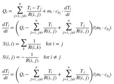
Finally, the most generic equation for thermal network solvers is derived below. Here, index 'i' is the node under iteration and 'j' refers nodes connected to it as described in node connectivity array, TA = ambient temperature, need not be same as RREF used for radiative heat transfer.
\(\sum\limits_{j} \left[ C_{ij} * (T_i - T_j) \right] + F_{ij} \cdot ε \cdot σ \cdot \sum\limits_{j} \left[ A_{ij} \cdot \left(\frac{(T_i + T_j)^4}{16} - T_{REF}^4 \right) \right] + \sum\limits_{j} \left[ h \cdot A_{ij} * \left( \frac{T_i + T_j}{2} - T_A \right) \right] = \dot{q}_i \)
\(\sum\limits_{j} \left[ C_{ij} * (T_i - T_j) \right] + F_{ij} \cdot ε \cdot σ \cdot \sum\limits_{j} \left[A_{ij} \cdot (\overline{T}_{ij}^2 - T_{REF}^2) \cdot (\overline{T}_{ij}^2 + T_{REF}^2) \right] + \sum\limits_{j} \left[h \cdot A_{ij} * \left(\frac{T_i + T_j}{2} - T_A\right) \right] = \dot{q}_i \)
Where \[\overline{T}_{ij} = \frac{T_i + T_j}{2}\]\(\sum\limits_{j} \left[ C_{ij} * (T_i - T_j) \right] + F_{ij} \cdot ε \cdot σ \cdot \sum\limits_{j} \left[A_{ij} \cdot (\overline{T}_{ij} - T_{REF}) \cdot (\overline{T}_{ij} + T_{REF}) \cdot (\overline{T}_{ij}^2 + T_{REF}^2) \right] + \sum\limits_{j} \left[h \cdot A_{ij} * (\overline{T}_{ij} - T_A) \right] = \dot{q}_i\)
\[ C_{RAD} = \underbrace{ (T_{REF}^2 + \overline{T}_{ij}^2) \cdot (\overline{T}_{ij} + T_{REF})}_\text{Non-linearity}\] \(\sum\limits_{j} \left[C_{ij} + F_{ij} ε \cdotσ \cdot \frac{A_{ij}}{2} \cdot C_{RAD} + h/2 \cdot A_{ij} \right ] \cdot T_i - \sum\limits_{j} \left(C_{ij} + F_{ij} ε \cdotσ \cdot \frac{A_{ij}}{2} \cdot C_{RAD} + h/2 \cdot A_{ij} \right) \cdot T_j = \dot{q}_i + \sum\limits_{j} F_{ij} \cdot ε \cdot σ \cdot A_{ij} \left[ T_{REF} \cdot C_{RAD} \right] + \sum\limits_{j} \left(h \cdot A_{ij} \cdot T_A \right) \)For 'i' defined in first column of node connectivity array above and 'j' varying from second column onwards for each 'i':
\[K_{ii}\cdot T_i + \sum\limits_{j}\left[K_{ij} \cdot T_j\right] = b_i \] where \[K_{ii} = \sum\limits_{j}\left[C_{ij} + F_{ij} ε \cdotσ \cdot \frac{A_{ij}}{2} \cdot C_{RAD} + h/2 \cdot A_{ij} \right ]\] \[ K_{ij} = - \left (C_{ij} + F_{ij} ε \cdotσ \cdot \frac{A_{ij}}{2} \cdot C_{RAD} + h/2 \cdot A_{ij} \right) \]Sample thermal network for a battery pack
                   [CON1+]        [CON1-]          [CON2+]         [CON2-]
                     |              |                 |               |
                     |__[Case-top]__|                 |___[Case-top]__|    ...other cells
                            |                                 |
                            |                                 |
                        [Cell-Z]                          [Cell-Z]
                            |                                 |
                            |                                 |
[Case]--[Gap-1]--[Can-1]--[C-1]--[Can-1]--[Gap-2]--[Can-2]--[C-2]--[Gap-3] ...other cells
                            |                                 |
                            |                                 |
                        [Cell-Z]                          [Cell-Z]
                            |                                 |
                            |                                 |
                        [Case-Bot]                        [Case-Bot]       ...other cells
TNSolver Examples
Most of the examples in public domain are available through work published by Bob Cochran at Applied Computational Heat Transfer, Seattle, WA (TNSolver@heattransfer.org). Not much could be found in other sources. From user guide: plane wall with fixed temperature and convection boundary conditions.|```````| [in] [out]---[Tinf] h = 2.3 [W/m2-K] | | ``````` Begin Solution Parameters title = Simple Wall Model type = steady units = SI T units = C !Default is 'C', other options K, F, R End Solution Parameters Begin Conductors ! label type nd_i nd_j parameters wall conduction in out 2.3 1.2 1.0 ! k L A fluid convection out Tinf 2.3 1.0 ! h A End Conductors Begin Boundary Conditions ! type parameter node(s) fixed_T 21.0 in ! Inner wall T fixed_T 5.0 Tinf ! Fluid T End Boundary ConditionsDetailed output is in *.out file. The *.rst file contains:
 time = 0
    in  21
   out  12.2727
  Tinf  5
*.csv files contain
"label", "type", "nd_i", "nd_j", "T_i (C)", "T_j (C)", "Q (W)", "U (W/m^2-K)", "A (m^2)"
"wall",  "conduction", "in",  "out",  21, 12.2727, 16.7273, 1.91667, 1
"fluid", "convection", "out", "Tinf", 12.2727, 5,  16.7273, 2.3, 1
and
"label", "material", "volume (m^3)", "temperature (C)"
"in",    "N/A", 0, 21
"out",   "N/A", 0, 12.2727
"Tinf",  "N/A", 0, 5
Solution of the sample case described above (and used for Python scripting), in TNSolver without convection at nodes: note that TNSolver has option of specified temperature, heat flux, heat source and volumetric heat source at nodes. Convection can be specified on resistors only. Thus, tip convection can be applied using additional node to represent T∞ or the reference temperature for HTC.
Begin Solution Parameters
  title   = Simple Wall Model
  type    = steady
  units   = SI
  T units = K            !Default is 'C', other options K, F, R
End Solution Parameters

Begin Conductors
! label  type        nd_i   nd_j   parameters
  R01    conduction  N_01   N_02   200  0.050  0.0005   ! k L A
  R02    conduction  N_02   N_03   200  0.025  0.0005   ! k L A
  R03    conduction  N_02   N_04   200  0.025  0.0005   ! k L A
  R04    conduction  N_02   N_05   200  0.125  0.0005   ! k L A
  R05    conduction  N_05   N_06   200  0.025  0.0005   ! k L A
  R06    conduction  N_05   N_07   200  0.025  0.0005   ! k L A
  R07    conduction  N_05   N_08   200  0.025  0.0005   ! k L A
  R08    conduction  N_08   N_09   200  0.025  0.0005   ! k L A
  R09    conduction  N_09   N_10   200  0.025  0.0005   ! k L A
End Conductors

Begin Boundary Conditions
! type      parameter   node(s)
  fixed_T   288         N_01
  fixed_T   323         N_06
  fixed_T   373         N_10
End Boundary Conditions

Begin Sources
  ! type  parameter(s)  node(s)
    Qsrc  50.0          N_02
    Qsrc  50.0          N_03
    Qsrc  50.0          N_04
End Sources
Calculated temperature values in [K] are:
 time = 0
 N_01  288.0
 N_02  355.9
 N_03  368.4
 N_04  368.4
 N_05  338.2
 N_06  323.0
 N_07  338.2
 N_08  349.8
 N_09  361.4
 N_10  373.0
The result using Python code developed above and without heat transfer coefficient boundary at any node is given below. The values match with TNSolver and also demonstrates the fact that the effect of heat loss through convection at tip is negligible.
[288.0 355.9 368.4 368.4 338.2 323.0 338.2 349.8 361.4 373.0]
Example taken from "TNSolver: An Open Source Thermal Network Solver for Octave or MATLAB" by Bob Cochran at Thermal & Fluids Analysis Workshop (TFAWS) 2016
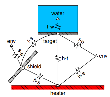
Begin Solution Parameters
  title = Radiation Heat Transfer Experiment - Black Target
  type  = steady
  nonlinear convergence = 1.0e-8
  maximum nonlinear iterations = 50
End Solution Parameters

Begin Conductors
  ! Conduction through the beaker wall, 0.1" thick pyrex glass
    t-bbin conduction targ bbin 0.14 0.00254 0.024829 ! k L A

  ! Convection from beaker to water
  ! label type        nd_i nd_j    mat     L       A
    t-w   ENChplateup bbin water   water   0.04445 0.02483

  ! Convection from target to air
  ! label type          nd_i   nd_j   mat  L       A
    t-air ENChplatedown targ   env    air  0.0889  0.0248

  ! Convection from outer shield to air
  ! label type          nd_i   nd_j   mat  H       L       theta  A
    s-air ENCiplateup   s_out  env    air  0.0508  0.0508  48.0   0.056439

  ! Conduction from inner to outer side of shield
    shield conduction s_in  s_out  steel  0.001   0.056439
End Conductors

Begin Radiation Enclosure
  ! surf   emiss  A        Fij
    htr    0.92   0.06701  0.0      0.1264   0.68415  0.0     0.1893
    targ   0.95   0.02482  0.34132  0.0      0.00603  0.1031  0.5494
    s_in   0.28   0.05643  0.81231  0.00265  0.12278  0.0     0.0622
    s_out  0.28   0.05643  0.0      0.0453   0.0      0.0     0.9546
    env    1.00   0.11840  0.10711  0.1151   0.02965  0.4547  0.2933
End Radiation Enclosure

Begin Boundary Conditions
  ! type     Tb     Node(s)
    fixed_T  23.0   env
    fixed_T  88.3   water
    fixed_T  515.0  htr
End Boundary Conditions
Output from *.rst file:
time = 0
bbin   93.4466
env    23
htr    515
s_in   272.032
s_out  271.956
targ   175.252
water  88.3
Fin with force convection and thermal radiation
                               [Tc]
                                |
            .,,,,,,,,,,,,,,,,,,,*,,,,,,,,,,,,,,,,,,,.      [Tc]
            |       |       |       |       |       |        |
            |       |       |       |       |       |        |
[base]-----[1]-----[2]-----[3]-----[4]-----[5]-----[6]-----[tip]
            |       |       |       |       |       |        |
            |       |       |       |       |       |        |
             ```````````````````|```````````````````       [Tr]
                              [Tr]

! Fin Experiment Model - Aluminum fin - Forced convection

Begin Solution Parameters
  title = Aluminum Fin - Forced Convection
  type                         = steady
  nonlinear convergence        = 1.0e-8
  maximum nonlinear iterations = 15
End Solution Parameters

Begin Conductors
! label type       nd_i  nd_j   k        L        A
  100  conduction  base   1   167.0    0.030    0.000127
  101  conduction   1     2   167.0    0.025    0.000127
  102  conduction   2     3   167.0    0.045    0.000127
  103  conduction   3     4   167.0    0.070    0.000127
  104  conduction   4     5   167.0    0.050    0.000127
  105  conduction   5     6   167.0    0.063    0.000127
  106  conduction   6    tip  167.0    0.002    0.000127

! label type      nd_i   nd_j mat  Vel   D        A
  121  EFCcyl      1     Tc   air  3.7  0.0127  0.00170
  122  EFCcyl      2     Tc   air  3.7  0.0127  0.00140
  123  EFCcyl      3     Tc   air  3.7  0.0127  0.00229
  124  EFCcyl      4     Tc   air  3.7  0.0127  0.00239
  125  EFCcyl      5     Tc   air  3.7  0.0127  0.00225
  126  EFCcyl      6     Tc   air  3.7  0.0127  0.00134
  127  EFCcyl     tip    Tc   air  3.7  0.0127  0.00013

! label type      nd_i   nd_j  emissivity     A
  221  surfrad     1     Tr      0.09    0.001696
  222  surfrad     2     Tr      0.09    0.001396
  223  surfrad     3     Tr      0.09    0.002294
  224  surfrad     4     Tr      0.09    0.002394
  225  surfrad     5     Tr      0.09    0.002254
  226  surfrad     6     Tr      0.09    0.001337
  227  surfrad    tip    Tr      0.09    0.000127
End Conductors

Begin Boundary Conditions
!  type        Tb      Node(s)
  fixed_T     25.0      Tc
  fixed_T     25.0      Tr
  fixed_T     55.8      base
End Boundary Conditions
Example of Composite Walls
     .---------,----------------------,-----------,
     |         |                      |           |
     |         |          kB          |           |
     |         |                      |           |
   [TIN]  kA  [1]--------------------[2]     kD  [TOUT]
     |         |                      |           |
     |         |          kC          |           |
     |_________|______________________|___________|

Option-1 of thermal network

             |````````|
             |        |
[TIN]-------[1]      [2]------[TOUT]
             |        |
             |        |
              ````````
! label type         node-1 node-2  parameters (k, L, A)
  100   conduction    Tin    1       1.0  1.0  2.0
  101   conduction    1      2       2.0  3.0  1.0
  102   conduction    1      2       2.0  3.0  1.0
  103   conduction    2      Tout    1.0  1.0  2.0


Option-2: Two parallel paths
  |`````````[1]``````[2]````````|
  |                             |
[TIN]                         [TOUT]
  |                             |
  |                             |
   `````````[3]``````[4]````````
! label type         node-1 node-2  parameters (k, L, A)
  100   conduction    Tin    1       1.0  1.0  1.0
  101   conduction    1      2       2.0  3.0  1.0
  102   conduction    2      Tout    1.0  1.0  1.0
  103   conduction    Tin    3       1.0  1.0  1.0
  104   conduction    3      4       2.0  3.0  1.0
  105   conduction    4      Tout    1.0  1.0  1.0
Fluid Network Solver
Many of the concepts used in thermal network solver can also be used in fluid network solver (without heat transfer). For incompressible flows (constant density), from continuity for node 'i' and connected nodes designated as 'j': \[\sum\limits_{j}Q_{ij} = Q_D \] where QD is flow demand (inflow or outflow) at node 'i'.Major difference is in the basic definitions though: ΔT = Q. RTH and ΔP = Q2 * RHD
If a flow network contains NN junctions (or nodes) then NN-1 independent continuity equations in the form given above can be written. A flow resistance network consisting of NN nodes (junctions) and NL non-overlapping loops formed by NP resistances, will satisfy the equation NP = (NN - 1) · NL. From energy equations in terms of head losses and NL number of independent loops, for loop 'i': \[\sum \limits_{j}\Delta h_{j}^i = 0 \] The head loss for a flow resistance is typically given as Δh = ξ·Qn (n = 2 for most cases): \[\sum \limits_{j}\xi_j \cdot Q_{j}^n = 0 \] Solving for the NP unknown volumetric flow rates in the NP flow resistances (pipes) of a network, as many number of equations must be derived. Most widely used method for solving fluid flow networks is the Hardy Cross method which is an adaptation of the Newton-Raphson method which solves one equation at a time before proceeding to the next equation during each iteration instead of solving all equations simultaneously. The steps used in Hardy-Cross method are as follows:- Make an initial guess of flow rates in each flow resistors
- Compute the sum of head losses around a loop of the network taking into account direction of flow: \(\sum \limits_{j}^{LOOP}\xi_j \cdot Q_{j}^n \)
- Calculate the sum of absolute values of differential of head loss equation: \(\sum \limits_{j}^{LOOP}\lvert n\cdot \xi_j \cdot Q_{j}^{n-1} \rvert \)
- Compute change in flow ΔQ by dividing results from step-2 by that of step-3.
- Repeat steps 2 to 4 for each loop in the flow network
- Repeat steps 2 to 5 iteratively until ΔQ computed during an iteration reduce below certain pre-defined tolerance (convergence criteria).
                [4]```````[5]``````[6]
                 |                  |
[1]-----[2]-----[3]                [7]
                 |                  |
                [8]-------[9]------[10]
                           |
                [12]------[11]-----[13]
                 |                  |
[17]-----------[14]                 |
                 |                  |
               [15]----------------[16]
And the input file can be of the following format where (like in thermal network solver) of '0' implies unknown (to be calculated). Note that NP = (NN - 1) · NL does not hold true here. For initial version of the solver, all nodes are assumed to be at same height. The hydraulic diameter, length and friction factor can be specified for each branch to calculate flow resistances. A friction factor of value 0 implies it is calculated as per empirical correlations, here correlations as per Swamee-Jain is used. A value of zero for hydraulic resistance implies that it needs to be calculated as per
\[R_1 = \frac{\Delta P}{\rho Q^2} = f \cdot \frac{L}{D} \cdot \frac{1}{2A^2} = \frac{1}{m^4}\]
\[R_1 = \frac{\Delta P}{\rho Q^2} = f \cdot \frac{8}{\pi^2} \cdot \frac{L}{D^5} = \frac{1}{m^4}\]
\[R_2 = \frac{\Delta h}{Q^2} = f \cdot \frac{8}{\pi^2} \cdot \frac{L}{D^5} = \frac{s^2}{m^3}\]
where A is the reference area or area based on hydraulic diameter. Note that hydraulic diameter DH, and wall roughness are in [mm], branch length L_BRANCH is in [m]. For pipe length 1.0 [m], diameter 250 [mm], to get R = 1.0, f = 1.205E-3
[FLOW RESISTORS BEGIN]
R_ID, s_node, e_node,  resistance,  fric_fac,   DH,    L_BRANCH, roughness
R01,       1,      2,      1.0,      0.02,      20.0,     100.0,    0.045
R02,       2,      3,      2.0,      0.02,      20.0,     100.0,    0.045
R03,       3,      4,      3.0,      0.02,      20.0,     100.0,    0.045
R04,       4,      5,      4.0,      0.02,      20.0,     100.0,    0.045
R05,       5,      6,      5.0,      0.02,      20.0,     100.0,    0.045
R06,       6,      7,      6.0,      0.03,      20.0,     100.0,    0.045
R07,       7,     10,      7.0,      0.02,      20.0,     100.0,    0.045
R08,       9,     10,      8.0,      0.01,      20.0,     100.0,    0.045
R09,       8,      9,      9.0,      0.01,      20.0,     100.0,    0.045
R10,       8,      3,      8.0,      0.01,      20.0,     100.0,    0.045
R11,       9,     11,      7.5,      0.02,      20.0,     100.0,    0.045
R12,      11,     12,      6.0,      0.01,      20.0,     100.0,    0.045
R13,      11,     13,      5.0,      0.01,      20.0,     100.0,    0.045
R14,      12,     14,      4.0,      0.01,      20.0,     100.0,    0.045
R15,      14,     15,      3.0,      0.05,      20.0,     100.0,    0.045
R16,      13,     16,      2.5,      0.01,      20.0,     100.0,    0.045
R17,      15,     16,      2.0,      0.02,      20.0,     100.0,    0.045
R18,      14,     17,      1.0,      0.01,      20.0,     100.0,    0.045
[FLOW RESISTORS END]
The nodes (junctions) of specified pressure and losses at junctions such as merging branches can be specified in following section. N_PR is pressure as node, N_SRC is momentum source or sink at the node (typically used at Tee and Y-junctions) - units same as pressure per unit denisty. Q_DMND is the demand (inflow or outflow) at the node, Q_BR is fixed flow through the branch. Note that pressure specified is in units of [J/kg] and not [Pa] - based on definition of flow resistance above.
[NODES BEGIN]
NNUM,      N_PR,   Q_DMND,  N_SRC
   1,       250,     1.50,  0
  17,         0,        0,  0
[NODES END]
Branches (hydraulic resistors with known fixed flow rates, or pump/fan curve). The specified flow rates should be in m3/s. The direction of flow should be from Node_i to Node_j. Q_BR acts as the constant in the fan curve C0 + C1*Q + C2*Q2.
[SPECIAL BRANCHES BEGIN]
Node_i, Node_j,   Q_BR, C1, C2
    13,     16,   0.05,  0,  0
[SPECIAL BRANCHES END]
Java Code to read the text file into dictionaries (data map) and vectors (list) as per pre-defined sections and headers. Sample input file is here.
def calcHydResistance(DH, LN, FF):
  # Calculate resistance (as per dP/ρ = R * Q^2) in units of [m-4]
  return (0.8105695 * LN * FF / D**5) # 8*FF*LN/π2/D5
Let's explore a generic branch connected with multiple branches at the two ends.
             [m]         [n]
              |           |
              |           |
      Qi---> [i]---------[j] <---Qj
             /            \
            /              \
           [u]             [v]
\( Q_i = R_{ij} \cdot (P_i - P_j)^n \text{ if } P_i > P_j\) where n = 1/2 for most of hydraulic elements. \( Q_j = R_{ij} \cdot (P_j - P_i)^n \text{ if } P_j > P_i\). In other words: \( Q_i = R_{ij} \cdot |P_i - P_j|^{n-1} \cdot (P_i - P_j)\) and \( Q_j = R_{ij} \cdot |P_j - P_i|^{n-1} \cdot (P_j - P_i)\). In matrix notation,
\[ \begin{bmatrix} Q_i \\ Q_j \end{bmatrix} = R'\begin{bmatrix} +1 \; \; -1 \\ -1 \; \; +1 \end{bmatrix} \begin{bmatrix} P_i \\ P_j \end{bmatrix} \dots [1] \]
Applying continuity at any interior node i (without mass generation or accumulation at any node, though mass can come in or go out from boundary nodes), a linear system of equations [R]{P'} = {Q*} can be created where vector {P'} is corrected pressure and vector {Q} is the estimated flow rates. This is an alternate formulation of element-by-element solution method which does not require formation of the full coefficient matrix. Conjugate Gradient method of solution can be used to iteratively solve the
linearised equations.
Instead of tracking sign of flow rates (direction), it is easier to use following formulation:
\[Q_{ij} = \frac{P_i - P_j}{|P_i - P_j|} \cdot \sqrt \frac{|P_i - P_j|}{R_{ij}} \dots [2]\] This can be conveniently implements in Python as: Q[i][j] = np.sign(P[i] - P[j]) * math.sqrt(abs(P[i] - P[j])/R[i][j])Another approach is to use SIMPLE-like algorithm used in 3D CFD simulation programs. The "true" pressure and flow rates are defined as \(P = P^{*} + P^{\prime }\) and \(Q = Q^{*} + Q^{\prime }\). By linearizing the momentum equation, the flow correction \(Q_{ij}^{\prime }\) is related to the pressure correction \(P^{\prime }\) by: \(Q_{ij}^{\prime }\approx d_{ij}(P_{i}^{\prime } - P_{j}^{\prime })\) where \(d_{ij}\) is a sensitivity coefficient derived from the derivative of the head loss equation. The quadratic head loss (\(\Delta P = R\cdot Q^{2}\)) is linearised using the derivative [dP/dQ]-1 = \(d = \frac{1}{2R\cdot Q}\)
Step-1: Guess initial values of pressures at nodes
Step-2: Calculate flow rates Q* through each branch using equation: \(P_i - P_j = \frac {Q_{ij}}{|Q_{ij}|} \cdot \xi_{ij}\frac{\rho}{2} \cdot \frac {Q_{ij}^2}{A^2}\) where Q/|Q| is a sign change term that insures that the pressure loss term always opposes the flow direction. For constant density and denoting P ≡ P/ρ, Q* ≡ QNEW = ΔP /(QOLD + ε) / R where R ≡ ξ/2A2 and Qij is the flow from node 'i' to node 'j' with appropriate sign.Step-3: Calculate flow rate correction Q' by differentiating branch pressure drop equation with respect to Qij where \(P'_i - P'_j = \frac {Q_{ij}}{|Q_{ij}|} \cdot R_{ij} \cdot Q_{ij}\)
\[\frac{dP_i}{dQ_{ij}} - \frac{dP_j}{dQ_{ij}} = 2 \cdot R_{ij} \cdot Q_{ij} \] dPi ≡ P'i | dPj ≡ P'j | dQi ≡ Q'i and dQj ≡ Q'j. Qij is flow through branch defined by nodes i and j, Qi is flow through branch number i. \[\frac{P'_i}{Q'_{ij}} - \frac{P'_j}{Q'_{ij}} = 2 \cdot R_{ij} \cdot Q_{ij} \] or \[\frac{P'_i}{\beta_{ij}} - \frac{P'_j}{\beta_{ij}} = Q'_{ij} \dots [3] \] where \[ \beta_{ij} = 2 \cdot R_{ij} \cdot Q_{ij} \] [1/βij] is the 'linearised' pipe conductance and the link to pressure-correction equations. The local slopes of pressure drop vs flow rate curve define linear mapping between pressure corrections to flow corrections (analogous to pressure correction schemes in CFD to enforce mass conservation by linearised momentum-pressure coupling).Step-4: Apply continuity equation at each node, excluding those at boundaries and known pressures to generate system of equation of the form [A]{P'} = {b}. Substitute \(Q_{ij} = Q_{ij}^{*} + Q_{ij}^{\prime }\) into the continuity equation at each node to obtain a system of linear equations for \(P^{\prime }\): \(\sum \limits_{j}d_{ij}(P_{i}^{\prime } - P_{j}^{\prime }) = S_{i} - \sum \limits_{j}Q_{ij}^{*} = b_i\). The right-hand side represents the mass imbalance (residual) at node 'i' and 1/βij ≡ dij
Step-5: Assemble the summation over all interior nodes to form the equation [A] · {P'} = {b} where diagonal terms Aii = Σkdik with 'k' denoting nodes connected to node 'i'. The off-diagonal terms are Aij = -dij where dij = 1/βij
Step-6: Solve for nodal values of P' and update nodal pressures, P = P* + P' and compute flow rates Q*ij
Step-7: Check for convergence of P' and Q* by checking maximum value in vector {b}
Step-8: Go to step-3 if convergence not achieved.
Improve robustness of convergence: Use under-relaxation factor (RF) for pressure correction p = p + RF * p' and limit the value of d when Q is closer to zero by capping 'Q' to small none zero value say 1.0E-5 [units].Newton-Raphson Method for One Non-Linear Equation
xi+1 = xi - f(x) / [∂f/∂x] - The Newton-Raphson method in matrix form to solve systems of non-linear equations, F(X) = 0, iteratively using the formula \(X_{n+1}=X_{n}-[J(X_{n})]^{-1}F(X_{n})\), where {X} is the vector of unknowns / variables, {F(X)} is the vector of functions, and [J(X)] is the Jacobian matrix containing all partial derivatives. At each iteration, it finds the change \(\Delta X=-[J(X_{n})]^{-1}F(X_{n})\) by solving a linear system, then updates the guess \(X_{n+1} = X_{n}+\Delta X\), repeating until convergence. Key Components System of Equations: \[F(X) = \left[\begin{matrix}f_{1}(x_{1},\dots , x_{n})\\ \vdots \\ f_{n}(x_{1},\dots ,x_{n})\end{matrix}\right]=\left[\begin{matrix}0\\ \vdots \\ 0\end{matrix}\right]\] Variables Vector: \[X = \left[\begin{matrix}x_{1}\\ \vdots \\ x_{n}\end{matrix}\right]\] Jacobian Matrix: \[J(X) = \left[\begin{matrix}\frac{\partial f_{1}}{\partial x_{1}}&\dots &\frac{\partial f_{1}}{\partial x_{n}}\\ \vdots &\ddots &\vdots \\ \frac{\partial f_{n}}{\partial x_{1}}&\dots &\frac{\partial f_{n}}{\partial x_{n}}\end{matrix}\right]\] Iteration Formula: \[X_{n+1} = X_{n}-[J(X_{n})]^{-1}F(X_{n})\] or \[X_{n+1} = X_{n} + \Delta X\text{, where }\Delta X = -[J(X_{n})]^{-1}F(X_{n})\]For more explanations, refer to page engcourses-uofa.ca/books/numericalanalysis/nonlinear-systems-of-equations/newton-raphson-method
Example network and coefficient matrix development
            (0)          (1)        (2)
 ---> [0]---->----[1]----->---[2]---->----[3] --->
       |           |                       |
       |           |                       |
       |          \|/(4)                  \|/(3)
       |           |                       |
       |           |          (6)          |
  (10)\|/         [4]---------->----------[5]
       |           |                       |
       |           |                       |
       |          \|/(8)                  \|/(5)
       |           |                       |
       |    (9)    |         (7)           |
      [8]----<----[7]---------<-----------[6] --->
From mass balance at each node:
+q[0] + q[1] + q[2] + q[3] + q[4] + q[5] + q[6] + q[7] + q[8] + q[9] + q[10] = b
--------------------------------------------------------------------------------
+q[0] +                                                       + q[10]        = qb[0]
-q[0] + q[1]               + q[4]                                            = 0
      - q[1] + q[2]                                                          = 0
             - q[2] + q[3]                                                   = qb[3]
                           - q[4]        + q[6]        + q[8]                = 0
                    - q[3]        + q[5] - q[6]                              = 0
                                  - q[5]        + q[7]                       = qb[6]
                                                - q[7] - q[8] + q[9]         = 0
                                                              - q[9] - q[10] = 0
The equations in matrix form is:
         0   1   2   3   4   5   6   7   8   9   10
Node  _               Resistor Numbers              _
  0  |  +1   0   0   0   0   0   0   0   0   0   +1  |  {q[0] }  = {qb[0]}
  1  |  -1  +1   0   0  +1   0   0   0   0   0    0  |  {q[1] }  = { 0   }
  2  |   0  -1  +1   0   0   0   0   0   0   0    0  |  {q[2] }  = { 0   }
  3  |   0   0  -1  +1   0   0   0   0   0   0    0  |  {q[3] }  = {qb[3]}
  4  |   0   0   0   0  -1   0  +1   0  +1   0    0  |  {q[4] }  = { 0   }
  5  |   0   0   0  -1   0  +1  -1   0   0   0    0  |  {q[5] }  = { 0   }
  6  |   0   0   0   0   0  -1   0  +1   0   0    0  |  {q[6] }  = {qb[6]}
  7  |   0   0   0   0   0   0   0  -1  -1  +1    0  |  {q[7] }  = { 0   }
  8  |   0   0   0   0   0   0   0   0   0  -1   -1  |  {q[8] }  = { 0   }
      ``                                            ``  {q[9] }
                                                        {q[10]}
How will the system of equations and matrix formulation change if a resistors say (6) is given fixed flow conditions? In other words, q[6] is known. Resistor (6) is defined by nodes [4] and [5] and hence q[6] term shall appear in mass balance equations for nodes [4] and [5]. Note that indices for nodes and hydraulic resistors follow different sequences.
The equations in matrix form shall translate into the following format:
         0   1   2   3   4   5   6   7   8   9   10
Node  _               Resistor Numbers              _
  0  |  +1   0   0   0   0   0   0   0   0   0   +1  |  {q[0] }  = {qb[0]}
  1  |  -1  +1   0   0  +1   0   0   0   0   0    0  |  {q[1] }  = { 0   }
  2  |   0  -1  +1   0   0   0   0   0   0   0    0  |  {q[2] }  = { 0   }
  3  |   0   0  -1  +1   0   0   0   0   0   0    0  |  {q[3] }  = {qb[3]}
  4  |   0   0   0   0  -1   0  (0)  0  +1   0    0  |  {q[4] }  = {-q[6]}
  5  |   0   0   0  -1   0  +1  (0)  0   0   0    0  |  {q[5] }  = {+q[6]}
  6  |   0   0   0   0   0  -1   0  +1   0   0    0  |  {q[6] }  = {qb[6]}
  7  |   0   0   0   0   0   0   0  -1  -1  +1    0  |  {q[7] }  = { 0   }
  8  |   0   0   0   0   0   0   0   0   0  -1   -1  |  {q[8] }  = { 0   }
      ``                                            ``  {q[9] }
                                                        {q[10]}
The variable q[6] shall not participate in iterative computation and hence A[u, NP_FF] = 0.0 and A[v, NP_FF] = 0 where 'u' and 'v' are the nodes defining the fixed flow branch number NP_FF. In this example, u = 4, v = 5 and NP_FF = 6.
The matrix equation in pressure form after linearisation Q[k] = (p[i] - p[j]) / R[k] / Q[k]
        0   1   2   3   4   5   6   7   8  9   10    {    dp     } / {REFF}       = {  b  }
Node _               Resistor Numbers             _
  0 |  +1   0   0   0   0   0   0   0   0   0   +1 | {p[0] - p[1]}/R[ 0]/Q[ 0] = {qb[0]}
  1 |  -1  +1   0   0  +1   0   0   0   0   0    0 | {p[1] - p[2]}/R[ 1]/Q[ 1] = { 0   }
  2 |   0  -1  +1   0   0   0   0   0   0   0    0 | {p[2] - p[3]}/R[ 2]/Q[ 2] = { 0   }
  3 |   0   0  -1  +1   0   0   0   0   0   0    0 | {p[3] - p[5]}/R[ 3]/Q[ 3] = {qb[3]}
  4 |   0   0   0   0  -1   0  +1   0  +1   0    0 | {p[1] - p[4]}/R[ 4]/Q[ 4] = { 0   }
  5 |   0   0   0  -1   0  +1  -1   0   0   0    0 | {p[5] - p[6]}/R[ 5]/Q[ 5] = { 0   }
  6 |   0   0   0   0   0  -1   0  +1   0   0    0 | {p[4] - p[5]}/R[ 6]/Q[ 6] = {qb[6]}
  7 |   0   0   0   0   0   0   0  -1  -1  +1    0 | {p[6] - p[7]}/R[ 7]/Q[ 7] = { 0   }
  8 |   0   0   0   0   0   0   0   0   0  -1   -1 | {p[4] - p[7]}/R[ 8]/Q[ 8] = { 0   }
     ``                                           `` {p[7] - p[8]}/R[ 9]/Q[ 9]
                                                     {p[0] - p[8]}/R[10]/Q[10]
     _                                            _
  0 |  +1   0   0   0   0   0   0   0   0   0   +1 | {p[0] - p[1]} / REFF00 = {qb[0]}
  1 |  -1  +1   0   0  +1   0   0   0   0   0    0 | {p[1] - p[2]} / REFF01 = { 0   }
  2 |   0  -1  +1   0   0   0   0   0   0   0    0 | {p[2] - p[3]} / REFF02 = { 0   }
  3 |   0   0  -1  +1   0   0   0   0   0   0    0 | {p[3] - p[5]} / REFF03 = {qb[3]}
  4 |   0   0   0   0  -1   0  +1   0  +1   0    0 | {p[1] - p[4]} / REFF04 = { 0   }
  5 |   0   0   0  -1   0  +1  -1   0   0   0    0 | {p[5] - p[6]} / REFF05 = { 0   }
  6 |   0   0   0   0   0  -1   0  +1   0   0    0 | {p[4] - p[5]} / REFF06 = {qb[6]}
  7 |   0   0   0   0   0   0   0  -1  -1  +1    0 | {p[6] - p[7]} / REFF07 = { 0   }
  8 |   0   0   0   0   0   0   0   0   0  -1   -1 | {p[4] - p[7]} / REFF08 = { 0   }
    ``                                            `` {p[7] - p[8]} / REFF09
                                                     {p[0] - p[8]} / REFF10
        _ 0   1   2   3   4   5   6   7   8 _
       | +1  -1   0   0   0   0   0   0   0  | {p[0]}
       |  0  +1  -1   0   0   0   0   0   0  | {p[1]}
       |  0   0  +1  -1   0   0   0   0   0  | {p[2]}
       |  0   0   0  +1   0  -1   0   0   0  | {p[3]}
{dp} = |  0  +1   0   0  -1   0   0   0   0  | {p[4]}  = [BT] * {p}
       |  0   0   0   0   0  +1  -1   0   0  | {p[5]}
       |  0   0   0   0  +1  -1   0   0   0  | {p[6]}
       |  0   0   0   0   0   0  +1  -1   0  | {p[7]}
       |  0   0   0   0  +1   0   0  -1   0  | {p[8]}
       |  0   0   0   0   0   0   0  +1  -1  |
       | +1   0   0   0   0   0   0   0  -1  |
       ``                                   ``
Here, REFF = R*Q. Note that vector {dp} can be formulated as [BT].{p} where {p} = {p[0] p[1] ... p[10]}T and hence {Q*} = {Δp}/{RQ} where right hand side is element-wise division.
As described in equation [3] above, it is pressure correction that is usually solved. The summary of steps in matrix notation is described again. Here · denotes matrix multiplication as per '@' operator in Python. * and / are element-wise multiplication and division of vectors.
- From continuity: [B] · {Q} = {Qd} where {Qd} is demand (outflow) or supply (inflow) at nodes
- As derived above, {Q*} = [B]T · {dp} / {REFF} where {REFF} = {R} · {Q*}
- As per linearisation: Q = Q* + Q' and hence {Q} = {Q*} + {Q'} where {Q*} is guessed or values calculated during iterations. Thus: residual vector or mass imbalance vector, [B]·{Q* + Q'} = {Qd}
- From iterative solution: {b} = {Qd} - [B] · {Q*}
- [B] · {Q'} = {Qd} - [B] · {Q*}
- [B] · {Q'} = {b}
- From equation (3) above: {Q'} = [1/β] · [dP'] = [1/β] · [B]T · {P'}
- From equations [B] · {Q'} = {b} and {Q'} = [1/β] · [B]T · {P'}
- [B] · [1/β] · [B]T · {P'} = {b}
- [Ap] · {P'} = {b}
- [Ap] = [B] · [1/β] · [B]T
- Note that {b} = - [B] · {Q*} where there is no external demand or supply at internal nodes.
Example Validation Cases
All resistances of equal diameters, density of working fluid = 1.25 [kg/m2 constant for all nodes. Resistances are in units of \(\frac{\Delta{P}}{\rho \cdot Q^2} = \frac{kg}{m.s^2}\cdot \frac{m^3}{kg} \cdot \frac{s^2}{m^6} = \frac{1}{m^4} \)Validation Case-1
[0]-------[1]-------[2]-------[3]
R_ID s_node e_node RHYD
R1   0      1      3
R2   1      2      5
R3   2      3      8
Specified pressure [Pa] nodes:
Node   N_PR
0      100
3      0
Flow through each branch = (100 / 16)0.5 = 2.5 [m3/s] and pressure drops are [18.75, 31.25, 50.0] Pa for each branch and hence node pressures are [100, 81.25, 50.0, 0.0] Pa.
Validation Case-2
[0]-------[1]-------[2]-------[3]
                     |
                     |
                    [4]
R_ID s_node e_node RHYD
R1   0      1      3
R2   1      2      5
R3   2      3      8
R3   2      4      2
Specified pressure [Pa] nodes:
Node   N_PR
0      100
3      0
4      0
For hydraulic resistance in parallel: \[\sqrt\frac{1}{R^{ij}_{EQ}} = \sqrt\frac{1}{R_i} + \sqrt\frac{1}{R_j} \] Nodes 3 and 4 are in parallel with respect to node 2. Overall resistance of the system = 3 + 5 + 0.889 = 8.889 and thus incoming flow at node 1 is (100 / 8.889)0.5 = 3.354 [m3/s] and pressure drops through series branches are [33.75, 56.25] Pa. The node 1 is at 100 - 33.75 = 66.25 [Pa] and node 2 is at 100 - [33.75 + 56.25] = 10.0 [Pa] and flow through branches 2-3 and 2-4 are [1.118, 2.236] [m3/s].
Solve "Validation Case-1" iteratively using manual (hand-calculation) method.
Step-1:
Initial value of p at nodes: [100, 0, 0, 0]Step-2:
Incidence Matrix: B[s_node, i] = +1 and B[e_node, i] = -1 for i = 0 to NP-1 ---as per assumption that flow along the left node to right node used to define branches (hydraulic resistances) is positive and flow in opposite direction is negative. If a node appears only as start node, it is assumed to have positive flow (flow shall enter into that node) and if a node appears only as end node, the flow is assumed to be negative (flow shall exit through that node).[[+1 0 0] [-1 +1 0] [ 0 -1 +1] [ 0 0 -1]]Each row of the incidence matrix defines the status of that node and node number of connected branches.
Step-3:
Initial flow rates through each branch: Q* = [5.770, 0.001, 0.001] using formula Q=[ΔP/R]1/2 or Q * Q = [ΔP/R] and hence Q = [ΔP/R/Q] then calculate mass imbalance for each node, {b} = [5.770 -5.770, 0.0, 0.0]Step-4:
Calculate pressure correction equation (coefficient matrix) - the right hand side of the equation is nothing but {b} which has unit of flow rate.
0.5 / (R[0][1] * Q[0][1]) * (P0' - P1')             =  Q*01
0.5 / (R[1][2] * Q[1][2]) *       (P1' - P2')       =  Q*12
0.5 / (R[2][3] * Q[2][3]) *             (P2' - P3') =  Q*23
or
1/β01|+1  -1   0   0| |P0'|    |b0|
1/β12| 0  +1  -1   0| |P1'| =  |b1|
1/β23| 0   0  +1  -1| |P2'|    |b2|
                      |P3'|
{βij} = (0.0289 = 0.5/5.770/3 100.0 = 0.5/0.001/5 62.5 = 0.5/0.001/8)
[A] =
[[  1       0          0        0   ]
 [  0       100.03   -100.0     0   ]
 [  0      -100.00    162.5     0   ]
 [  0       0          0        1   ]]
Step-5:
Solver p_corr = np.linalg.solve(A, b) which gives p_corr = [ 0 -0.150 -0.092 0] - note that pressure correction is negative and it will make intermediate pressure values at nodes beyond the lower and upper limits of boundary conditions. This is an example where {b} and [A] are calculated incorrectly. The iterations using Python code indeed diverged. One likely reason might be that the rows and columns corresponding for specified node pressure are part of coefficient matrix. Second, p_corr = np.linalg.solve(A, -b) should be used instead of p_corr = np.linalg.solve(A, b). In this case, p_corr = np.linalg.solve(A, -b) worked with same coefficient matrix [A] defined above. In MATLAB, mldivide (the backslash operator, A\B) solves the system of linear equations [A]{x} = {b} for vector {x}.Few properties of matrix multiplications
Multiplying a matrix by a diagonal matrix scales its rows or columns: left-multiplication (Diagonal Matrix * Base Matrix) scales each row of the matrix by the corresponding diagonal element, while right-multiplication (Base Matrix * Diagonal Matrix) scales each column by the corresponding diagonal element, effectively transforming the matrix without changing its dimensions.Multiplying a matrix [A] by a diagonal matrix [D] and then by the transpose of the first matrix [AT] results in a new symmetric matrix, where the elements across the main diagonal are equal, effectively scaling the rows of [A] by diagonal elements before combining them with the scaled columns of [AT].
Associativity of multiplication: A · (B · C) = (A · B) · C
Basic Fluid Network Solver: Both the node pressures and flow rates though branches match the hand calculations for the "Validation Case-1". You may test the following code for your application and let me know cases where it fails.
import numpy as np
def tupleToList(list_of_tuples):
  '''
  Return the length of unique items in a tuple defining branches
  '''
  list_1, list_2 = [], []
  for t in list_of_tuples:
    list_1.append(t[0])
    list_2.append(t[1])
  unique_list = list(set(list(set(list_1)) + list(set(list_2))))
  unique_list.sort()
  return len(unique_list), list_1, list_2

def pipeNetwork(pipes, pr_bc, alpha_p=0.5, alpha_q=0.7, max_iter=500, tol=1e-5):
  '''
  SIMPLE algorithm for arbitrary pipe networks with non-linear resistances
  and multiple pressure boundary conditions. Parameters are:
    pipes: list of (m, n, R) - Pipe from m -> n with resistance R
    pr_bc: dictionary - {node_index: pressure_value}
  '''
  eps = 1e-5
  Np = len(pipes)
  nn_nodes, ni, nj = tupleToList(pipes)
  nn_uknown = nn_nodes - len(pr_bc.items())

  # Incidence matrix
  B = np.zeros((nn_nodes, Np))  # N_nodes x N_branch = rows x cols
  R = np.zeros(Np)

  # Initial guess for pressures at nodes
  p = np.ones(nn_nodes)
  for node, val in pr_bc.items():
    p[node] = val
  Q = np.ones(Np) * 0.001   # small non-zero initial flow

  for i, (m, n, Ri) in enumerate(pipes):
    B[m, i] = +1.0
    B[n, i] = -1.0
    R[i] = Ri
    if p[m] - p[n] != 0:
      Q[i] = np.sign(p[m] - p[n]) * np.sqrt(abs(p[m] - p[n]) / R[i])

  # Start SIMPLE-type iterations
  for iter in range(max_iter):

    # 1. Update effective resistance (non-linearity)
    R_eff = R * np.abs(Q) + eps

    # 2. Momentum predictor
    dp = B.T @ p

    Q_star = dp / R_eff  # Q * Q = dp/R, Q = dp / [R * Q] = dp/R_eff

    # 3. Mass imbalance
    b = B @ Q_star

    # 4. Pressure correction system: dp/dq = 2RQ = 0.5/R_eff
    d = 0.5 / R_eff
    Ap = B @ np.diag(d) @ B.T

    # Apply pressure boundary conditions
    for node, val in pr_bc.items():
      Ap[node, :] = 0.0
      Ap[:, node] = 0.0
      Ap[node, node] = 1.0
      b[node] = 0.0

    # 5. Solve pressure correction: "source term" is the mass imbalance
    p_corr = np.linalg.solve(Ap, -b)

    # 6. Update pressures
    p = p + alpha_p * p_corr
    for node, val in pr_bc.items():
      p[node] = val

    # 7. Correct flows
    for i, (m, n, Ri) in enumerate(pipes):
      if p[m] - p[n] != 0:
        Q[i] = np.sign(p[m] - p[n]) * np.sqrt(abs(p[m] - p[n]) / R[i])

    # 8. Check convergence: return node connectivity, node pressure, flow rates
    if np.max(np.abs(b)) < tol:
      print(f"Converged in {iter + 1} iterations.")
      return ni, nj, p, Q

  # Print divergence and return 'None'
  print("SIMPLE did not converge!")
  return ni, nj, None, None

pipes = [(0, 1, 3.0), (1, 2, 5.0), (2, 3, 8.0), (2, 4, 2.0)]
pr_bc = {0: 100.0, 3: 0.0, 4: 0.0}

ni, nj, nodeP, Qdot = pipeNetwork(pipes=pipes, pr_bc=pr_bc, max_iter=100)
if nodeP is not None:
  print("-" * 50)
  print("All values are in chosen unit of pressure and [m^3/s]")
  print("Node pressures:")
  for index, value in enumerate(nodeP, start=1):
    print(f"{index}: {value:8.2f}")

if Qdot is not None:
  print("-" * 50)
  print("Flow through pipe branches:")
  for index, value in enumerate(Qdot):
    print(f" {ni[index]} -> {nj[index]} = {value:6.3f}  |", end="")
print("\n")
Here pipe or branch data is represented as tuple (as definition of branch required > 2 variables) and node data as dictionaries (key-value pair can be used to define nodes). This code is part of category known as Gradient Method because it contains gradient of pressures in the pipe branches. The flow correction is proportional to the negative gradient of energy (pressure) imbalance. Ap = B @ np.diag(d) @ B.T is analogous to a Hessian matrix. Due to symmetry, positive definite and sparse nature of coefficient matrix, algorithm is numerically strong (fast and relatively robust).
This code does not provide option to specify fixed flow rate through a branch. The code solves incompressible flow (constant density) and pressure is in reality specific energy [J/kg] - where hydraulic resistance is defined ΔP/ρ = R.Q2. There are some constraint to this simple program: all boundary nodes (those connected with only one other node) has to be specified pressure boundary conditions, even if it is zero. The interior nodes can have known pressures. Pump or fans cannot be modeled (specifying two nodes with fixed pressure increase shall not work).How to implement inflow / outflow nodes and fixed flow resistors?
Note that two boundary nodes connected to an internal node should not have different boundary conditions such as fixed pressure on one and fixed outflow on another. The equation ΔP = R.Q2 will not satisfy on both the branches.To implement inflow or outflow boundary conditions: update vector {b} in SIMPLE iteration such that b[i] = b[i] - Q[i] for node 'i' where Q is positive when flow enters into the flow network through that node. A check is required to ensure same boundary node is not specified pressure as well as inflow / outflow value.
To implement flow demand and supply at nodes, flow rates through branches do not need to be directly adjusted to meet demand. Instead, 'demand' modifies node continuity equation and solver should automatically adjust branch flows using head changes. Once residuals (vector 'b' above) has been calculated for each node without considering demand as each node, create a loop over all nodes and update values of b[i] based on flow demand and sign convention adopted (outflow + or -).For branches with fixed flow rates, update flow correction section in SIMPLE iteration as per following conditions. Here ff_resistances is the list of tuples defining start node, end node and fixed flow rate values. Let's assume node j and k constitute the branch with fixed flow - these nodes cannot be the boundary node (else it will contradict the boundary conditions at these nodes).
          (j)        (k)         (m)
-----[a]-------[u]--------[v]--------[b]-------
                |          |
             (r)|          |(s)
                |          |
               [c]        [d]
-q[j] + q[k] + q[c]                =  0
      - q[k] +      q[s] + q[m]    =  0
or
-q[j] +        q[c]                = -q[k]
                    q[s] + q[m]    = +q[k]
Practically, the nodes defining both the fixed flow branch and pressure jump or fan branch behave like boundary nodes. In case of fixed flow branch, the pressures at node 'u' and node 'v' are decided by the upstream and downstream conditions respectively where outflow at 'u' = inflow at 'v', the pressure drop through fixed-flow branch has no practical value.
In case of fixed flow branch, the incidence matrix needs to be updated as B[u, k] = 0.0 = B[v, k] where 'k' is the branch number defined above. Additionally, the "Flow Correction" section needs to be added with following conditions.
if u == m and v == n:
  Q[i] = Q_k
for k, (u, v, Q_k) in enumerate(ff_branches):
  b[u] = b[u] + Q_k
  b[v] = b[v] - Q_k
In case of pressure jump boundary conditions (which implies a fixed pressure difference exists between two nodes regardless of flow), outflow at 'u' = inflow at 'v' and p[v] = p[u] + Δp. For pressure jump or fan boundary conditions, it is mandatory to use two-branched nodes (those connected with exactly two branches) such as -----[u]---Δp---[v]----- The method requires to find the branch numbers connected to nodes 'u' and 'v' and apply same flow rates to all the 3 branches in addition to p[v] = p[u] + Δp. The flow through the branch defining the pressure jump does not need to be solved same as in fixed-flow branch case. Since pressure of downstream node is known with respect to upstream node, the pressure at downstream node does not need to be solved a part of matrix inversion.
          (j)        (k)         (m)
-----[a]-------[u]--------[v]--------[b]-------
-q[j] + q[k]        = 0
      - q[k] + q[m] = 0
 q[j]               = +q[k]
 q[m]               = +q[k]
For better convergence, use q[k] = (q[j] + q[m])/2.0 and the flow rate calculation for branch 'j' and 'm' needs an update on sign convention for pressure drop.
To implement a second order polynomial for fans where p[v] = p[u] + C0 + C1 * Q[k] + C2 * Q[k]**2, method similar to pressure jump can be updated by adding C1 * Q[k] + C2 * Q[k]**2 as C0 is already modeled in pressure jump.
Calculate resistance based on hydraulic diameter, flow rate and roughness: if the flow resistance is specified as zero, a function can be used to calculate friction factor based on empirical correlations and then calculate hydraulic resistance.
The formula is \[f = \frac{0.25}{\left[\log _{10}\left(\frac{\epsilon }{3.7D} + \frac{5.74}{\text{Re}^{0.9}}\right)\right]^{2}}\] where ε is absolute roughness, D is pipe diameter, and Re is the Reynolds number.def ffSwameeJain(dia, e, Re): return 0.25 / (math.log10(e / 3.7 / dia + 5.74 / Re**0.9))**2The comparison between iterative (implicit) Colebrook-White formula and non-iterative (explicit) Swamee-Jain correlation (at roughness height 0.045) is shown below ↴


Checks for User Inputs: some basic checks are necessary to ensure user inputs are as per expected format. Checks like duplicate branch, same branch with nodes in reverse order, missing node (branch defined by only one node), two different type of boundary conditions defined for same node and node number in boundary conditions not defined in the branch definitions can be easily done in few lines of code.
The printable version of method described above can be accessed here.
Picard-type element (pipe-based) iterations are another algorithm to solve pipe networks which avoid full Newton-Raphson type Jacobians and instead solve a linearised system using updated element conductances at every outer iteration.Quality Assurance of Flow Network Solvers
One approach to validate the output is to check the results by switching boundary conditions at same node. With node-0 applied to 100 [Pa] pressure for validation case-2 described above, the calculated values are summarized below. All boundary nodes are set to pressure value of 0 [Pa] unless a non-zero value is specified in dictionary pr_bc.
Case with pressure boundary conditions - no inflow/outflow:
pipes = [(0, 1, 3.0), (1, 2, 5.0), (2, 3, 8.0), (2, 4, 2.0)]
pr_bc = {0: 100}
All values are in [J/kg] and [m^3/s]
Node pressures:
0:   100.00
1:    66.25
2:    10.00
3:     0.00
4:     0.00
--------------------------------------------------
Flow through pipe branches:
 0 -> 1 = 3.3541  | 1 -> 2 = 3.3541  | 2 -> 3 = 1.1180  | 2 -> 4 = 2.2361  |
Case with outlet pressure boundary and inflow:
pipes = [(0, 1, 3.0), (1, 2, 5.0), (2, 3, 8.0), (2, 4, 2.0)]
pr_bc = {}
ff_bc = {0: 3.354}
The output is:
All values are in [J/kg] and [m^3/s]
Node pressures:
0:    99.99
1:    66.25
2:    10.00
3:     0.00
4:     0.00
--------------------------------------------------
Flow through pipe branches:
 0 -> 1 = 3.3540  | 1 -> 2 = 3.3540  | 2 -> 3 = 1.1180  | 2 -> 4 = 2.2360  |
Case with pressure boundary conditions and fixed flow branch:
Inputs:
pipes = [(0, 1, 3.0), (1, 2, 5.0), (2, 3, 8.0), (2, 4, 2.0), (3, 5, 1.0)]
pr_bc = {0:100, 5:0}   # Nodes with pressure boundary conditions
ff_bc = {}             # Inflow / outflow nodes
ff_branches = [(2, 3, 2.5)]

Results:
All values are in [J/kg] and [m^3/s]
Node pressures:
0:   100.00
1:    63.25
2:     2.00
3:     6.25
4:     0.00
5:     0.00
--------------------------------------------------
Flow through pipe branches:
 0 -> 1 = 3.5000  | 1 -> 2 = 3.5000  | 2 -> 3 = 2.5000  | 2 -> 4 = 1.0000  |
 3 -> 5 = 2.5000  |
Flow network with fixed-flow and fan boundary conditions
pipes = [(0, 1, 11.95), (1, 2, 5.0), (2, 3, 8.0), (2, 4, 2.0),
         (3, 5, 1.0), (1, 6, 7.5), (6, 7, 1.0), (7, 8, 5.0)]
ff_rs = [(2, 3, 1.0)]   # Fixed flow branch
pj_rs = [(6, 7, 20)]    # Pressure jump branch
pr_bc = {0:100}
          PFAN = 20
       6-----------7-----------8
       |
 0-----1-----2-----4
             |
             3
             |
             5
Results are:
Converged in 22 iterations
--------------------------------------------------
All values are in [J/kg] and [m^3/s]
Node pressures:
0:   100.00
1:     8.20
2:     0.15
3:     1.00
4:     0.00
5:     0.00
6:    -8.72
7:    11.28
8:     0.00

--------------------------------------------------
Flow through pipe branches:
  0 -> 1 = 2.7716  | 1 -> 2 = 1.2695  | 2 -> 3 = 1.0000  | 2 -> 4 = 0.2695  |
  3 -> 5 = 1.0000  | 1 -> 6 = 1.5021  | 6 -> 7 = 1.5021  | 7 -> 8 = 1.5021  |
One of the simplest example to test the solver on pipe network with pressure jump branch can be one shown below.
 p=100        dp=20            p=0
 0---------1---------2---------3
     R=3       R=1       R=5
Flow rate through each branch = [120/8]0.5 = 3.873 [units]. Pressure values at nodes shall be [100]------[55]------[75]------[0]. Here, the pressure jump acts as pressure booster for node 2. If the pressure jump direction is reversed, flow rate reduces to [80/8]0.5 = 3.162 [units] and pressure values at nodes shall be [100]-----[70]-----[50]-----[0].
Another validation case from Hydraulics of Pipeline Systems, Example problem 4.6 is described below. The pipe network has 2 pumps, two globe valves and a meter and fluid is water at 10 [°C].
            0.030
             /|\
              |
  6----(7)----1-----(1)----2------> 0.080
170 [m]       |            | \
              |            |   \
             (4)          (2)   (5)
              |            |       \
              |            |         \
  7----(8)----4-----(3)----3----(6)---5---> 0.080
200 [m]                    |
                           |
                          \|/
                         0.050

Branch   Diameter [mm]   Length [m]
 1        200             500
 2        200             300
 3        200             500
 4        200             300
 5        200             500
 6        200             500
 7        250             300
 8        250             300
Branch number and flow rates [m3/s]: 1 → 2: 0.103, 3 → 2: 0.014, 4 → 3: 0.107, 4 → 1: 0.078, 2 → 5: 0.037, 3 → 5: 0.043, 6 → 1: 0.055, 7 → 4: 0.185
Example: 3-Reservoirs System, here \(R=\frac{8fL}{\pi^{2}gD^{5}}\)
Goal is to find the flow in each of the three pipes and the pressure at the junction '4' and pressure is expressed as height of water column.
|       |
|  [1]  |             |       |
|_______|             |  [3]  |
   \           /``````|_______|
    \         /
     \       /
      \     /
       \   /             |       |
        \ /              |  [2]  |
      [4]*---------------|_______|
          \
           \
===========---=====================Ground==========
H = (70   80  100   ?) [m], friction factor = 0.015
L[1, 4] =  5000 [m], L[2, 4] = 3000 [m], L[3, 4] = 4000 [m]
D[1, 4] =  0.60 [m], D[2, 4] = 0.80 [m], D[3, 4] = 1.20 [m]
R[1, 4] = 72.7266,   R[2, 4] = 11.3517 , R[3, 4] = 1.99316

Pipe [1, 4]: H[1] - H[4] = R[1, 4] * Q[1, 4] * |Q[1, 4]|
Pipe [2, 4]: H[2] - H[4] = R[2, 4] * Q[2, 4] * |Q[2, 4]|
Pipe [3, 4]: H[3] - H[4] = R[3, 4] * Q[3, 4] * |Q[3, 4]|

Pipe [1, 4]:  70 = H[4] + 72.7266 * Q[1, 4] * |Q[1, 4]|
Pipe [2, 4]:  80 = H[4] + 1.99316 * Q[2, 4] * |Q[2, 4]|
Pipe [3, 4]: 100 = H[4] + 11.3517 * Q[3, 4] * |Q[3, 4]|
From continuity (mass conservation) at node-4: Q[1, 4] + Q[2, 4] + Q[3, 4] = 0. Re-arranging the 4 equations:
H[4]    R[1, 4]*Q[1, 4]*|Q[1, 4]|               0                           0               = 70
H[4]                0               R[2, 4]*Q[2, 4]*|Q[2, 4]|                           0   = 100
H[4]                0                           0               R[3, 4]*Q[3, 4]*|Q[3, 4]|   = 80
   0            Q[1, 4]                     Q[2, 4]                     Q[3, 4]             = 0
The system is non-linear and needs an iterative solution method. The conventional vector-matrix format is:
[1    R[1, 4]*|Q[1, 4]|                    0                     ] {H[4]   }    {H[1]}   {e1}
[1                    0    R[2, 4]*|Q[2, 4]|                     ] {Q[1, 4]} _  {H[2]} = {e2}
[1                    0                    0    R[3, 4]*|Q[3, 4]|] {Q[2, 4]}    {H[3]}   {e3}
[0                    1                    1                    1] {Q[3, 4]}    {   0}   {e4}
Right-hand side of the system of equations is a vector of continuity (mass imbalances). One method to solve them is to square these values eTe (T = transpose), then minimize this sum of squared errors by changing unknowns "H[4], Q[1, 4], Q[2, 4], Q[3, 4]" to get the solution.
Results are: Q[1, 4] = -0.395 [m3/s] i.e. 0.395 [m3/s] from node 4 to reservoir 1 (opposite the original assumed direction), Q[2, 4] = +1.273 [m3/s] from reservoir 2 to the node 4 (along the assumed flow direction in the pipe), Q[3, 4] = -0.890 [m3/s] i.e. 0.890 [m3/s] from the node 4 to reservoir 3 (opposite the original assumed direction) and h[4] = 81.60 [m] with mass imbalance of -0.012 [m3/s] at node '4'.
The input for the pipeNetwork() program described above would be as mentioned below. Note that the pressure of reservoirs should be as per equation P = ρgh. However, for demonstration purpose, the pressure was specified as P/ρ/g which is "pressure head" and hence output pressure for node '0' is also in this unit only.pipes = [(0, 1, 72.7266), (0, 2, 11.3517), (0, 3, 1.99316)]
pr_bc = {1: 70.0, 2: 100.0, 3: 80.0}
And output from the program is:
Converged in 18 iterations
--------------------------------------------------
All values are in chosen unit of pressure and [m^3/s]
Node pressures:
1:    81.53
2:    70.00
3:   100.00
4:    80.00
--------------------------------------------------
Flow through pipe branches:
 0 -> 1 =  0.398  | 0 -> 2 = -1.275  | 0 -> 3 =  0.877  |
Helper Functions to Develop the Solver in Java
Note that Java is Objects-only and a strongly typed language which requires all variables to be declared before use. There is no implicit variable type like in Python and the equivalent code in Java would require much more lines of code. Read this section to get more summary of Java macros in STAR-CCM+ software. Additional example of functions and methods can be found here.The steps used to create a pipe network solver are:
- Define branch and node input text / csv files. Python code above uses lists and dictionaries. The Java code below uses classes for Branches and Nodes.
- Create functions and class/methods to store them in arrayLists (lists and dictionaries in Python)
- Get the number of nodes and list of nodes from branch data (such as tupleToList function above), note that the node dictionary (or list) in Python and class in Java contains information only related to boundary conditions.
- Write function or method to get boundary condition values (pressure and flow demand) at nodes.
- Define interim variables such as list for pressure at nodes, pressure drop in branches, flow rates in branches, relaxation factors...
- Initialize pressure values at nodes and write a function to assign boundary conditions at nodes during each iteration.
- Create a function to iterate till convergence is reached.
Read branch information in CSV file and carry out some operations. The BranchRecord class creates getter functions for headers defined in branch_data.csv file.
public class BranchRecord {
  private String branch_id, branch_type;
  private int start_node, end_node;
  private float resistance, add_param;

  public BranchRecord(String branch_id, int start_node, int end_node,
    float resistance, String branch_type, float add_param) {
    this.branch_id = branch_id;
    this.start_node = start_node;
    this.end_node = end_node;
    this.resistance = resistance;
    this.branch_type = branch_type;
    this.add_param = add_param;
  }

  // Getters and potentially setters
  public String getBranch_id() {
    return branch_id;
  }
  public int getStart_node() {
    return start_node;
  }
  public int getEnd_node() {
    return end_node;
  }
  public float getResistance() {
    return resistance;
  }
  public String getBranch_type() {
    return branch_type;
  }
  public float getAdd_param() {
    return add_param;
  }
}
Java method to get unique values from a 2D arrayList: here 'Branch' is the name of class to define data for branches.
  public static List<Integer> getNodesList(List<Branch> br_list) {
    List<Integer> node_list = new ArrayList<>();
    Set<Integer> branch_nodes = new HashSet<>();
    for (Branch row : br_list) {
       branch_nodes.add(row.s_node);
       branch_nodes.add(row.e_node);
    }
    node_list.addAll(branch_nodes);
    Collections.sort(node_list);

    return node_list;
  }
The following class reads CSV file and process it. Note that the string value for branch type in .CSV file should be without double quotes.
import java.io.BufferedReader;
import java.io.FileReader;
import java.io.IOException;
import java.util.ArrayList;
import java.util.List;

public class CsvReaderProcessor {
  public static void main(String[] args) {
    String csvFile = "data_branches.csv";
    String line;
    String cvsSplitBy = ",";
    List<BranchRecord> records = new ArrayList>>();

    try (BufferedReader br = new BufferedReader(new FileReader(csvFile))) {
      // Skip the header line if your CSV has one
      br.readLine();

      while ((line = br.readLine()) != null) {
        String[] data = line.split(cvsSplitBy);

        // CSV format: branch_id, start_node, end_node, resistance, branch_type, param_x
        if (data.length >= 4) {
          try {
            String br_id = data[0].trim();
            int s_node = Integer.parseInt(data[1].trim());
            int e_node = Integer.parseInt(data[2].trim());
            float hyd_res = Float.parseFloat(data[3].trim());
            String br_type = data[4].trim();
            float add_param = Float.parseFloat(data[5].trim());
            records.add(new BranchRecord(br_id, s_node, e_node, hyd_res, br_type, add_param));
          } catch (NumberFormatException e) {
            System.err.println("Skipping line due to invalid number format: " + line);
          }
        }
      }
    } catch (IOException e) {
      e.printStackTrace();
    }
    System.out.println("Number of branches: " + records.size());

    // Now perform operations based on string value
    processBranch(records, "FFlow");
  }
  public static void processBranch(List records, String br_type) {
    float ff_branch_r  = 0.0f;
    float ff_branch_dp = 0.0f;
    float ff_branch_q  = 0.0f;
    int count = 0;

    for (BranchRecord record : records) {
      if (record.getBranch_type().equalsIgnoreCase(br_type)) {
        ff_branch_q  = record.getAdd_param();
        ff_branch_dp = record.getResistance() * ff_branch_q * ff_branch_q;
        count++;
      }
    }

    System.out.println("\nOperations for branch type: " + br_type);
    if (count > 0) {
      System.out.println("dP for fixed flow branch: " + ff_branch_dp + " [Pa]");
    } else {
      System.out.println("No records found for " + br_type);
    }
  }
}
Sample CSV file
branch_id, s_node, e_node, resistance, branch_type, add_param
B01,       0,      1,      5.0,        Pipe,        0.0
B02,       1,      2,      3.0,        Pipe,        0.0
B03,       2,      3,      2.0,        FFlow,       0.5
B04,       3,      4,      1.0,        Pipe,        0.0
Output from Java Code
Number of branches: 4

Operations for branch type: FFlow
dP for fixed flow branch: 0.5 [Pa]
Create a vector (Python list) from 2D arrayList - this can be used to create lists of each column in Branch class. In the example below <T> implies that the vector can consists of any type such as integer, double or string.
import java.util.ArrayList;
import java.util.List;
import java.util.Vector;

public class arrayListToVector {

  public static <T> Vector<T> createVectorFromColumns(List> data,
    int[] columnIndices) {
    Vector<T> resultVector = new Vector<>();

    // Iterate through each row in the 2D ArrayList
    for (List<T> row : data) {
      // Iterate through each specified column index
      for (int colIndex : columnIndices) {
        // Ensure row has enough columns to avoid an IndexOutOfBoundsException
        if (colIndex >= 0 && colIndex < row.size()) {
          resultVector.add(row.get(colIndex));
        } else {
          // Handle cases where a row is shorter than the requested column index
          System.err.println("Warning: Column index " + colIndex +
            " out of bounds for a row of size " + row.size());
        }
      }
    }
    return resultVector;
  }
  public static void main(String[] args) {
    // Example usage
    List<List<String>> dataTable = new ArrayList<>();
    dataTable.add(List.of("A1", "1", "C1"));
    dataTable.add(List.of("A2", "2", "C2"));
    dataTable.add(List.of("A3", "3", "C3"));

    // Extract column indices 1 (A column) and 2 (C column)
    int[] columnsToExtract = {0, 2};
    Vector<String> extractedVector1 = createVectorFromColumns(dataTable, columnsToExtract);
    System.out.println("Extracted Vector: " + extractedVector1);

    int[] columnToExtract = {1};
    Vector<String> extractedVector2 = createVectorFromColumns(dataTable, columnToExtract);
    System.out.println("Extracted Vector: " + extractedVector2);
  }
}
Calculates the total count of unique elements across two given lists. The method below uses Set which automatically handles uniqueness and addAll method in HashSet which ignores any duplicates already present in the set. It returns size of the set, the total count of unique values.
import java.util.Arrays;
import java.util.HashSet;
import java.util.List;
import java.util.Set;
import java.util.Vector;

public class getUniqueItemCount {

  public static <T> int countUniqueValues(Vector<T> list_1, Vector list_2) {
    Set<T> uniqueElements = new HashSet<>(list_1);
    uniqueElements.addAll(list_2);
    return uniqueElements.size();
  }
  public static void main(String[] args) {
    List<Integer> s_node = Arrays.asList(1, 2, 3);
    Vector<Integer> vector_s_node = new Vector<>(s_node);
    List<Integer> e_node = Arrays.asList(2, 3, 4);
    Vector<Integer> vector_e_node = new Vector<>(e_node);

    int uniqueCount = countUniqueValues(vector_s_node, vector_e_node);
    System.out.println("Total unique values: " + uniqueCount);
  }
}
The example case with pressure boundary conditions was solved using Java code and result matches with Python code. Note the higher number of iterations required.
Input: Branch data in branches.csv where Branch class is defined as public Branch(int id, int s_node, int e_node, String br_type, double resistance, double add_param). Here, add_param is used to specify flow rate for Fixed Flow branch, δp for pressure jump branch. The resistance and additional parameters together can be used to define fan curve in the form A + B * Q + C *Q2 where Q is flow rate through the branch. Refer the example with "Fixed-Flow and Pressure Jump" in later sections.
id, s_node, e_node, br_type, resistance, add_param
0,   0,     1,      PIPE,    3.0,        0
1,   1,     2,      PIPE,    5.0,        0
2,   2,     3,      PIPE,    8.0,        0
3,   2,     4,      PIPE,    2.0,        0
Input: Node data in nodes.csv where Node class is defined as public Node(int id, double pressure, double Qdemand).
id, pressure, Qdemand
0,  100,      0
3,  0,        0
4,  0,        0
Solver: the solver class contains functions to read nodes, branches, get node list from branch information, get list of boundary nodes defined in nodes.csv and function to iterate till mass-balance at each node is satisfied. It does not use matrix assembly operation and function like np.linalg.solve(A, b).
Output
Converged in 149 iterations
Node pressures [J/kg]:
Node id: 0, Node Pressure:  100.000
Node id: 1, Node Pressure:   66.250
Node id: 2, Node Pressure:   10.000
Node id: 3, Node Pressure:    0.000
Node id: 4, Node Pressure:    0.000

Branch flows [m^3/s]:
Branch ID: 0, Branch Flow Rate:   3.3541
Branch ID: 1, Branch Flow Rate:   3.3541
Branch ID: 2, Branch Flow Rate:   1.1180
Branch ID: 3, Branch Flow Rate:   2.2361
For use of NumPy like library in Java, one need to install Efficient Java Matrix Library (EJML). It is a linear algebra library for manipulating real / complex / dense / sparse matrices. EJML is free, written in 100% Java and has been released under an Apache v2.0 license. It has a function solve(A,B) which returns the solution {x} from [A]*{x} = {B}.
Example case with Fixed-Flow and Pressure Jump
The flow network with fixed-flow and pressure-jump boundary conditions above has been solved using the Java code - the friction factor and diameter was chosen such that they result in hydraulic resistance of 10.0 [m-4] for branch 0. For diameter 250 [mm] and length 1.0 [m], friction factor required to get resistance of 10 [m-4] is 0.01205.As explained earlier, the value of 0 for resistance implies that it should be calculated based on friction factor, diameter and length of the pipe. If friction factor is also specified 0, it would be calculated as per Swamee-Jain correlation and then hydraulic resistance shall be calculated.
Click the tabs below to get inputs used for Branches and Nodes.
#id, s_node, e_node, br_type, resistance, fric_factor, pipe_len, pipe_dia, roughness
#                    PJMP,    0.0,        C0,           C1,       C2
#                    FANC,    0.0,        C0,           C1,       C2
#                    FFLO,    0.0,        Qdot,
 0,   0,     1,      PIPE,    0.0,        0.0144,       1.000,    250.0,    0.04
 1,   1,     2,      PIPE,    5.0,        0.00,         1.000,    10.0,     0.04
 2,   2,     3,      FFLO,    8.0,        1.00,         1.000,    10.0,     0.04
 3,   2,     4,      PIPE,    2.0,        0.00,         1.000,    10.0,     0.04
 4,   3,     5,      PIPE,    1.0,        0.00,         1.000,    10.0,     0.04
 5,   1,     6,      PIPE,    7.5,        0.00,         1.000,    10.0,     0.04
 6,   6,     7,      PJMP,    1.0,        20.0,         1.000,    10.0,     0.04
 7,   7,     8,      PIPE,    5.0,        0.00,         1.000,    10.0,     0.04
# Specify -1 for pressure if Qdemand is to be applied at an internal node
# id, pressure, Qdemand
  0,  100,      0
  4,  0,        0
  5,  0,        0
  8,  0,        0
# Values are in SI unit (temperature in degree C)
op_pressure    = 101325.0
op_temperature = 25.0
material_name  = air
viscosity      = 1.86e-5
density        = 1.20
max_iter       = 1000
conv_crit      = 1.0e-5
Converged in 104 iterations
---------------------
Node pressures [J/kg]:
Node id:  0, Pressure:  100.000
Node id:  1, Pressure:    8.202
Node id:  2, Pressure:    0.145
Node id:  3, Pressure:    1.000
Node id:  4, Pressure:    0.000
Node id:  5, Pressure:    0.000
Node id:  6, Pressure:   -8.719
Node id:  7, Pressure:   11.281
Node id:  8, Pressure:    0.000

Branch flows [m^3/s]:
Branch  0 |   0  ->   1:   2.7713
Branch  1 |   1  ->   2:   1.2694
Branch  2 |   2  ->   3:   1.0000
Branch  3 |   2  ->   4:   0.2695
Branch  4 |   3  ->   5:   1.0000
Branch  5 |   1  ->   6:   1.5020
Branch  6 |   6  ->   7:   1.5021
Branch  7 |   7  ->   8:   1.5021
Now, friction factor based on flow rate (2.7714 m3/s), diameter 250 [mm], length 1.0 [m], density (1.2 kg/m3), viscosity (1.86E-5 Pa.s), and roughness (0.04 mm) is estimated as f = 0.0144. Corresponding flow resistance is 11.95 [m-4.
The default values for density and viscosity coded in the main program are 1.0 [kg/m3] and 1.0E-5 [Pa.s]. The next improvement is to read common data such as density, viscosity, operating temperature... from a Common.dat file. To read data from a file in one method and use it in another method within the same Java class, the first method should read the data and return it as a data structure like a Map<String, Double>, which is then passed as an argument to the second method. The following code will not store values like material_name = air, the entries in the file should be in the format String = Double such as density = 1.20 to specify constant (mean) density. The 3 methods defined below (readDataFromFile, getMatPropList and getMatProps) are required to update default values of density and viscosity.
import java.io.IOException;
import java.nio.file.Files;
import java.nio.file.Path;
import java.nio.file.Paths;
import java.util.List;
import java.util.HashMap;
import java.util.Map;

public class ReadCommonData {
  public static double mu;
  public static double rho;

  public static List<String> readDataFromFile(String file_name) throws IOException {
    Path path = Paths.get(file_name);
    return Files.readAllLines(path);
  }
  public static Map<String, Double> getMatPropList(List<String> dataLines) {
    Map<String, Double> common_data = new HashMap<>();
    for (String line : dataLines) {
      if (line.trim().isEmpty() || line.trim().startsWith("#"))
        continue;
      // Split the line by '=' character
      String[] parts = line.split("=", 2);
      if (parts.length == 2) {
        String value_str = parts[1].trim();
        if (!value_str.matches("[a-zA-Z]+")) {
          double value = Double.parseDouble(value_str);
          common_data.put(parts[0].trim(), value);
        }
      }
    }
    return common_data;
  }
  public static void getMatProps() {
    String file_name = "Common.dat";
    try {
      List<String> lines = readDataFromFile(file_name);
      Map<String, Double> mat_prop = getMatPropList(lines);
      mu  = mat_prop.get("viscosity");
      rho = mat_prop.get("density");
    } catch (IOException e) {
      System.err.println("Error handling file: " + e.getMessage());
      e.printStackTrace();
    }
  }
  public static void main(String[] args) {
    ReadCommonData mat_props = new ReadCommonData();
    mat_props.getMatProps();
    // Without %f, following line shall print "viscosity = " only
    System.out.printf("Viscosity = %f \n", mu);
  }
}
Common.dat contains following lines of text:
fluid_name = air
viscosity  = 1.86e-5
density    = 1.187
The validation of FAN curve to reproduce the result with pressure jump boundary condition of 20 [J/kg] has been achieved by using the equation 21.7 + 3.75 * flow - 3.25 * flow * flow thus using C0 = 21.7, C1 = 3.75 and C2 = -3.25 for coefficients. Note that the keyword 'FANC' is used to represent 'PUMP' also. Keywords PJMP or FANC can be used represent control valves where loss coefficients are similar functions of flow rate.
Note that there is no check of negative pressure head developed at higher flow rates as per the fan curve. Hence, fan curve should be inline with expected flow rate in the system. Similarly, there is no check for validity of entered inputs or missing inputs. However, following method or something similar can be used to sanitize the inputs.
public class CleanNumbers {
  public static Double cleanDouble(String str_input) {
    String str_cleaned = str_input;
    if (str_input != null && str_input.length() > 0) {
      if (str_input.contains("--"))
        str_cleaned = str_input.replace("--", "-");
      if (str_cleaned.contains(".."))
        str_cleaned = str_cleaned.replace("..", ".");

      if (str_cleaned.endsWith("-"))
        str_cleaned = str_cleaned.substring(0, str_cleaned.length() - 1);

      // Remove all characters except digits, dots, and minus signs
      // [^0-9.-] means: NOT (digit, dot, or minus)
      str_cleaned = str_cleaned.replaceAll("[^0-9.-]", "");

    } else {
      return null;
    }
    try {
      return Double.parseDouble(str_cleaned);
    } catch (NumberFormatException e) {
      return 0.0;
    }
  }
  public static void main(String[] args) throws Exception {
    System.out.println(cleanDouble("-123..5--"));
    // Output = -123.5
  }
}
User Guide and Limitation of this Network Solver
Step-1: Create the network diagram of the computational domain with nodes and branches named without any gap (continuous numbering) - refer the sample layouts aboveStep-2: Create the Branches.csv file - note the file name must be 'Branches.csv' - copy the sample input above, duplicate rows and update as needed. Alternatively, create the Branches.csv file using this page.
Step-3: Create the nodes.csv file - note the file name must be 'Nodes.csv' - copy the sample input above, duplicate rows and update as needed
Step-4: Create the Common.dat file - note the file name must be 'Common.dat' - copy the sample input above and update as needed
Step-5: Save all the 3 text files and 3 Java classes in same folder - open terminal and change current working directory to this folder
Step-6: Run command "java PipeNetworkSolver" from the command prompt.
Limitations
- Only incompressible fluid implemented as of now - implementation of gas properties as per ideal gas law in progress
- No checks on correctness of the inputs from users such as duplicate nodes or branches, missing values
- Comments cannot be put on the data line (they can be put on a new line starting with #)
- Viscosity needs to be specified - no internal calculation based on type of fluid
- Inflexible file names and variable names - they must be as mentioned above
- No heat transfer modeled or impact of heating/cooling of fluids.
Sample Code based on Picard Iterations
The Java code containing all classes and inputs in same file can be accessed here. The output produced by this code is included below.Iter 10, max |dQ|=1.996e-06 maxKCL=1.468e-06 Converged in 16 iterations. max|dQ|=8.191e-09, maxkCL=6.013e-09 ---=== Pressures at Nodes ===---===---==. Node 0: head = +120.000 m (-fixed) | demand= +0.0000 m^3/s Node 1: head = +44.011 m (solved) | demand= -0.0010 m^3/s Node 2: head = +9.335 m (solved) | demand= +0.0000 m^3/s Node 3: head = +0.000 m (-fixed) | demand= +0.0000 m^3/s ---=== Flow through Branches ===---===--* Branch ID : Flow Rate | Pressure Drop | Picard slope -------------:--------------------|-----------------|---------------- Link 0 (0->1): Q = +0.00308 m^3/s | dP = +75.989 | C(Qk) = 2.5e+04 Link 1 (1->2): Q = +0.00208 m^3/s | dP = +34.677 | C(Qk) = 1.7e+04 Link 2 (2->3): Q = +0.00208 m^3/s | dP = +9.335 | C(Qk) = 2.1e+03
Hardy-Cross Method Example:
A single closed loop with three pipes (Pipe 1, Pipe 2, Pipe 3) and known flow in a main supply line. The head loss (\(h_{f}\)) can be calculated using the Darcy-Weisbach equation in its discharge form: \(h_{f}=R\cdot Q^{2}\), where \(R=\frac{8fL}{\pi ^{2}gD^{5}}\) is the pipe resistance coefficient. 'R' values are known and constant. A clockwise flow is positive, and counter-clockwise is negative.Step 1: Assign Initial Flow Rates (Q) and R values
Pipe   Length (L)   Diameter (D)   Friction Factor (f)   Resistance (R)  Flow (Q)
  1    ...             ...              ...              0.5             10
  2    ...             ...              ...              0.8             6
  3    ...             ...              ...              1.2             4
Note: Ensure the initial flow guess satisfies continuity at junctions.
Step 2: Calculate the Head Loss hf for each pipe The head loss is \(h_{f} = R\cdot Q|Q|\) to maintain the correct sign for head loss regardless of flow direction. Pipe 1: \(h_{f1}=R_{1}\cdot Q_{1}|Q_{1}| = 0.5\cdot 10\cdot 10 = +50\), Pipe 2: \(h_{f2} = R_{2}\cdot Q_{2}|Q_{2}| = 0.8\cdot 6\cdot 6 = +28.8\), Pipe 3: \(h_{f3} = R_{3}\cdot Q_{3}|Q_{3}| = 1.2\cdot (-4)\cdot |-4|= -19.2\) (Negative because flow is counter-clockwise)
Step 3: Check the Head Loss Summation around the loop According to energy conservation, the sum of head losses around a closed loop should be zero (\(\sum h_{f}=0\)). \(\sum h_{f} = h_{f1} + h_{f2} + h_{f3} = 50 + 28.8 + (-19.2) = 59.6\) The result is not zero, so the initial flow rates are incorrect.
Step 4: Calculate the Flow Correction ΔQ. The Hardy-Cross method uses the following formula to find the flow correction needed for the loop: \(\Delta Q = -\frac{\sum h_{f}}{n\sum (\frac{h_{f}}{Q})}\) where n is typically 2. Calculate \(\sum (\frac{h_{f}}{Q})\) (absolute values can be used here as the sign is handled in the \(h_{f}\) summation). Pipe 1: \(\frac{h_{f1}}{Q_{1}} = \frac{50}{10} = 5\), Pipe 2: \(\frac{h_{f2}}{Q_{2}} = \frac{28.8}{6} = 4.8\), Pipe 3: \(\frac{h_{f3}}{Q_{3}} = \frac{-19.2}{-4} = 4.8\), \(\sum (\frac{h_{f}}{Q}) = 5 + 4.8 + 4.8 = 14.6\) Now, calculate \(\Delta Q\): \(\Delta Q = -\frac{59.6}{2\cdot 14.6} = -\frac{59.6}{29.2}\approx -2.04\)Step 5: Update the Flow Rates Apply the flow correction to each pipe in the loop. The sign of \(\Delta Q\) is negative, meaning the flows in the clockwise direction were overestimated and need to be reduced, or the counter-clockwise flow needs to be increased. Pipe 1 (Clockwise): \(Q_{1,new} = Q_{1} + \Delta Q = 10 + (-2.04) = 7.96\), Pipe 2 (Clockwise): \(Q_{2,new} = Q_{2} + \Delta Q = 6 + (-2.04) = 3.96\), Pipe 3 (Counter-clockwise, so subtract \(\Delta Q\)): \(Q_{3,new} = Q_{3}-\Delta Q = -4-(-2.04) = -1.96\)
Step 6: Repeat Repeat the process (Steps 2-5) with the new flow rates until the ΔQ value is negligible (close to zero), indicating that \(\sum h_{f}\) is close to zero and the solution has converged. The process is iterative and can be automated using spreadsheets or scripting such as Python programming.References:
- Textbook of Heat Transfer by S.P. Sukhatme
- Numerical Heat Transfer and Fluid Flow by Suhas V Patankar
- Introduction to Fluid Mechanics and Fluid Machines by S. K. Som, Gautam Biswas, and S. Chakraborty
- A New Approach to Modeling Fluid/Gas Flows in Networks by W. S. Winters, SANDIA REPORT SAND2001-8422
- Algorithms for Pipe Network Analysis and Their Reliability by Don J. Wood, University of Kentucky
- Pipe Network Analysis By Mun-Fong Lee, University of Florida, Gainesville
- A robust simulator of pressure-dependent consumption in Python by Camille Chambon et. al.
- Hydraulics of Pipeline Systems by Bruce E. Larock, Rowland W. Jeppson, Gary Z. Watters
The content on CFDyna.com is being constantly refined and improvised with on-the-job experience, testing, and training. Examples might be simplified to improve insight into the physics and basic understanding. Linked pages, articles, references, and examples are constantly reviewed to reduce errors, but we cannot warrant full correctness of all content.
Template by OS Templates