- Artificial Intelligence, Machine Learning, Python, Web Scraping: Feedbacks/Queries -

Artificial Intelligence
Machine Learning Methods and Scripts
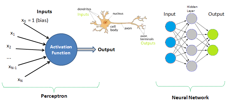
Table of Contents
- Regression and Logistic Regression (GNU OCTAVE) [*] Linear Algebra ---Principal Component Analysis (*) PCA (GNU OCTAVE) {*}K-Nearest Neighbours (KNN) using Python + sciKit-Learn --- clustering by K-means (GNU OCTAVE) ---Probability in Machine Learning [+] Optimization Methods and Algorithms
- SVM using Python + sciKit-Learn --- Naive Bayes classification --- Anomaly Detection --- Recommender Systems and Collaborative Filtering --- Decision Tree / Random Forest Classification with Python + sciKit-Learn
- Python install / update -|- OCTAVE vs. Python -|- Python Argument Parsing | Vectorization | Arrays / Slicing of Arrays || OOP in Python -|- Web Scraping in Python -|- Tuple and Dictionaries |:| Pandas |-| File Operations in Python [/] Computer Vision
Human Brain: Have you tried to search online the keywords "number of neurons in the brain"? The answer is invariably 100 billions! There is another data that we use only 1% of brain and hence do the number 1 billion neurons not astonish you? Can we build a machine and the learning algorithm to deal with similar number of neurons?
What to Expect On This Page
Each statement is commented so that you easily connect with the code and the function of each module - remember one does not need to understand everything at the foundational level - e.g. the linear algebra behind each algorithm or optimization operations! The best way is to find a data, a working example script and fiddle with them.

✍Machine learning, artificial intelligence, cognitive computing, deep learning... are emerging and dominant conversations today all based on one fundamental truth - follow the data. In contrast to explicit (and somewhat static) programming, machine learning uses many algorithms that iteratively learn from data to improve, interpret the data and finally predict outcomes. In other words: machine learning is the science of getting computers to act without being explicitly programmed every time a new information is received.
An excerpt from Machine Learning For Dummies, IBM Limited Edition: "AI and machine learning algorithms aren't new. The field of AI dates back to the 1950s. Arthur Lee Samuels, an IBM researcher, developed one of the earliest machine learning programs - a self-learning program for playing checkers. In fact, he coined the term machine learning. His approach to machine learning was explained in a paper published in the IBM Journal of Research and Development in 1959". There are other topics of discussion such as Chinese Room Argument to question whether a program can give a computer a 'mind, 'understanding' and / or 'consciousness'. This is to check the validity of Turing test developed by Alan Turing in 1950. Turing test is used to determine whether or not computer (or machines) can think (intelligently) like humans.
| Feature | Data Engineer | Data Analyst | Data Scientist |
| Primary Focus | Build systems and pipelines | Insight generation and Reporting | Predictive modeling and ML |
| Data Focus | Raw/Unstructured Data | Historical/Structured Data | Complex/Predictive Data |
| Key Tools | SQL, Python, ETL, Spark, Cloud | SQL, Tableau/PowerBI, Excel | Python, R, ML, SQL, AI |
| Output | Data Pipelines and Data Warehouse | Dashboards and Business Insights | Predictions and ML Models |
The technical and business newspapers/journals are full of references to "Big Data". For business, it usually refers to the information that is capture or collected by the computer systems installed to facilitate and monitor various transactions. Online stores as well as traditional bricks-and-mortar retail stores generate wide streams of data. Big data can be and are overwhelming consisting of data table with millions of rows and hundreds if not thousands of columns. Not all transactional data are relevant though! BiG data are not just big but very often problematic too - containing missing data, information pretending to be numbers and outliers.
◎Data Management
Data management is art of getting useful information from raw data generated within the business process or collected from external sources. This is known as data science and/or data analytics and/or big data analysis. Paradoxically, the most powerful growth engine to deal with technology is the technology itself. The internet age has given data too much to handle and everybody seems to be drowning in it. Data may not always end up in useful information and a higher probability exists for it to become a distraction. Machine learning is related concept which deals with Logistic Regression, Support Vector Machines (SVM), k-Nearest-Neighbour (KNN) to name few methods.
Before one proceed further, let's try to recall how we were taught to make us what is designated as an 'educated or learned' person (we all have heard about literacy rate of a state, district and the country).
| Classical Learning Method | Example | Applicable to Machine Learning? |
| Instructions: repetition in all 3 modes - writing, visual and verbal | How alphabets and numerals look like | No |
| Rule | Counting, summation, multiplication, short-cuts, facts (divisibility rules...) | No |
| Mnemonics | Draw parallel from easy to comprehend subject to a tougher one: Principal (Main), Principle (Rule) | Yes |
| Analogy | Comparison: human metabolic system and internal combustion engines | No |
| Inductive reasoning and inferences | Algebra: sum of first n integers = n(n+1)/2, finding a next digit or alphabet in a sequence | Yes |
| Theorems | Trigonometry, coordinate geometry, calculus, linear algebra, physics, statistics | Yes |
| Memorizing (mugging) | Repeated speaking, writing, observing a phenomenon or words or sentences, meaning of proverbs | Yes |
| Logic and reasoning | What is right (appropriate) and wrong (inappropriate), interpolation, extrapolation | Yes |
| Reward and punishment | Encourage to act in a certain manner, discourage not to act in a certain manner | Yes |
| Identification, categorization and classification | Telling what is what! Can a person identify a potato if whatever he has seen in his life is the French fries? | Yes |
This is just a demonstration (using Python and scikit-learn) of one out of many machine learning methods which let users know what to expect as someone wants to dive deeper. One need not understand every line of the code though comments have been added to make the readers grab most out of it. The data in CSV format can be downloaded from here.
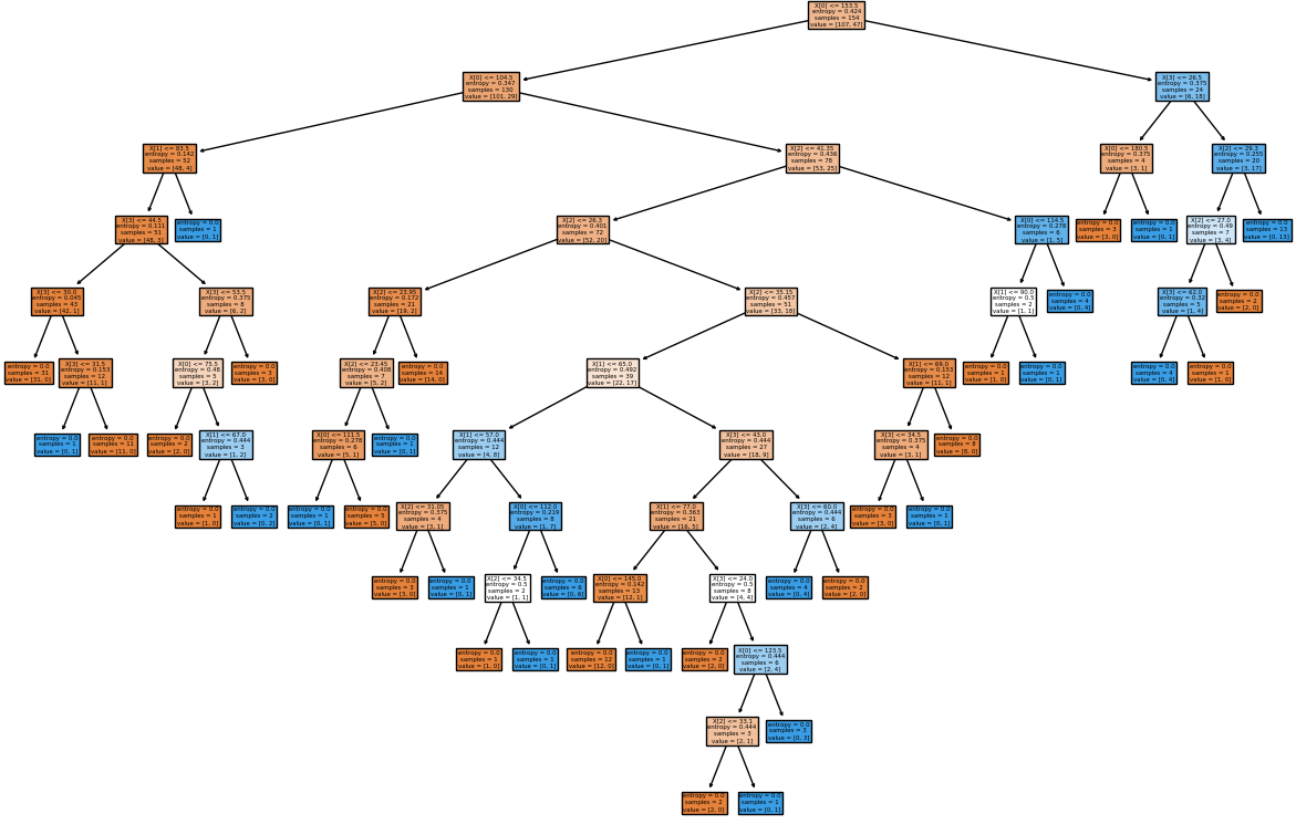
#      CLASSIFICATION: 'DECISION TREE' USING PYTHON + SCIKIT-LEARN

#On WIN10, python version 3.5
#Install scikit-learn: C:\WINDOWS\system32>py.exe -m pip install -U scikit-learn
#pip install -r list.txt - install modules (1 per line) described in 'list.txt'

# Decision Tree method is a 'supervised' classification algorithm.
# Problem Statement: The task here is to predict whether a person is likely to
# become diabetic or not based on 4 attributes: Glucose, BloodPressure, BMI, Age

# Import numPy (mathematical utility) and Pandas (data management utility)
import numpy as np
import pandas as pd
import matplotlib.pyplot as plt

# Import train_test_split function from ML utility scikit-learn for Python
from sklearn.model_selection import train_test_split

#Import scikit-learn metrics module for accuracy calculation
from sklearn import metrics

#Confusion Matrix is used to understand the trained classifier behavior over the
#input or labeled or test dataset
from sklearn.metrics import confusion_matrix
from sklearn.metrics import accuracy_score
from sklearn.metrics import classification_report

from sklearn import tree
from sklearn.tree import DecisionTreeClassifier, plot_tree
from sklearn.tree.export import export_text
# Import dataset: header=0 or header =[0,1] if top 2 rows are headers
df = pd.read_csv('diabetesRF.csv', sep=',', header='infer')

# Printing the dataset shape
print ("Dataset Length: ", len(df))
print ("Dataset Shape: ", df.shape)
print (df.columns[0:3])
# Printing the dataset observations
print ("Dataset: \n", df.head())

# Split the dataset after separating the target variable
# Feature matrix
X = df.values[:, 0:4] #Integer slicing: note columns 1 ~ 4 only (5 is excluded)
#To get columns C to E (unlike integer slicing, 'E' is included in the columns)

# Target variable (known output - note that it is a supervised algorithm)
Y = df.values[:, 4]

# Splitting the dataset into train and test
X_trn, X_tst, Y_trn, Y_tst = train_test_split(X, Y, test_size = 0.20,
    random_state = 10)
#random_state: If int, random_state is the seed used by random number generator
#print(X_tst)

#test_size: if 'float', should be between 0.0 and 1.0 and represents proportion
#of the dataset to include in the test split. If 'int', represents the absolute
#number of test samples.  If 'None',  the value is set to the complement of the
#train size. If train_size is also 'None', it will be set to 0.25.
# Perform training with giniIndex.  Gini Index is a metric to measure how often
# a randomly chosen element would be incorrectly identified (analogous to false
# positive and false negative outcomes).

# First step: #Create Decision Tree classifier object named clf_gini
clf_gini = DecisionTreeClassifier(criterion = "gini", random_state=100,
    max_leaf_nodes=3, max_depth=None, min_samples_leaf=3)

#'max_leaf_nodes': Grow a tree with max_leaf_nodes in best-first fashion. Best
#nodes are defined as relative reduction in impurity. If 'None' then unlimited
#number of leaf nodes.

#max_depth = maximum depth of the tree. If None, then nodes are expanded until
#all leaves are pure or until all leaves contain < min_samples_split samples.

#min_samples_leaf = minimum number of samples required to be at a leaf node. A
#split point at any depth will only be considered if it leaves at least
#min_samples_leaf training samples in each of the left and right branches.

# Second step: train the model (fit training data) and create model gini_clf
gini_clf = clf_gini.fit(X_trn, Y_trn)

# Perform training with entropy, a measure of uncertainty of a random variable.
# It characterizes the impurity of an arbitrary collection of examples. The
# higher the entropy the more the information content.
clf_entropy = DecisionTreeClassifier(criterion="entropy", random_state=100,
    max_depth=3, min_samples_leaf=5)
entropy_clf = clf_entropy.fit(X_trn, Y_trn)
# Make predictions with criteria as giniIndex or entropy and calculate accuracy
Y_prd = clf_gini.predict(X_tst)

#y_pred = clf_entropy.predict(X_tst)

#-------Print predicted value for debugging purposes ---------------------------
#print("Predicted values:")
#print(Y_prd)

print("Confusion Matrix for BINARY classification as per sciKit-Learn")
print("    TN   |    FP   ")
print("-------------------")
print("    FN   |    TP   ")
print(confusion_matrix(Y_tst, Y_prd))

# Print accuracy of the classification = [TP + TN] / [TP+TN+FP+FN]
print("Accuracy = {0:8.2f}".format(accuracy_score(Y_tst, Y_prd)*100))

print("Classification Report format for BINARY classifications")
#                           P           R           F           S
#                       Precision     Recall      fl-Score    Support
#       Negatives (0)   TN/[TN+FN]    TN/[TN+FP]  2RP/[R+P]   size-0 = TN + FP
#       Positives (1)   TP/[TP+FP]    TP/[TP+FN]  2RP/[R+P]   size-1 = FN + TP
# F-Score = harmonic mean of precision and recall - also known as the Sorensen–
# Dice coefficient or Dice similarity coefficient (DSC).
# Support = class support size (number of elements in each class).
print("Report: ", classification_report(Y_tst, Y_prd))

''' ---- some warning messages -------------- ------------- ---------- ----------
Undefined Metric Warning: Precision and F-score are ill-defined and being set to
0.0 in labels with no predicted samples.
- Method used to get the F score is from the "Classification" part of sklearn
- thus it is talking about "labels".  This means that there is no "F-score" to
calculate for some label(s) and F-score for this case is considered to be 0.0.
'''

#from matplotlib.pyplot import figure
#figure(num=None, figsize=(11, 8), dpi=80, facecolor='w', edgecolor='k')
#figure(figsize=(1,1)) would create an 1x1 in image = 80x80 pixels as per given
#dpi argument.

plt.figure()
fig = plt.gcf()
fig.set_size_inches(15, 10)

clf = DecisionTreeClassifier().fit(X_tst, Y_tst)
plot_tree(clf, filled=True)

fig.savefig('./decisionTreeGraph.png', dpi=100)
#plt.show()
#---------------------- ------------------------ ----------------- ------------
#Alternate method to plot the decision tree is to use GraphViz module
#Install graphviz in Pyhton- C:\WINDOWS\system32>py.exe -m pip install graphviz
#Install graphviz in Anaconda: conda install -c conda-forge python-graphviz
#---------------------- ------------------------ ----------------- ------------
Data management is the method and technology of getting useful information from raw data generated within the business process or collected from external sources. Have you noticed that when you search for a book-shelf or school-shoes for your kid on Amazon, you start getting google-ads related to these products when you browse any other website? Your browsing history is being tracked and being exploited to remind you that you were planning to purchase a particular type of product! How is this done? Is this right or wrong? How long shall I get such 'relevant' ads? Will I get these ads even after I have already made the purchase?
The answer to all these questions lies in the way "data analytics" system has been designed and the extent to which it can access user information. For example, are such system allowed to track credit card purchase frequency and amount?
Related fields are data science, big data analytics or simply data analytics. 'Data' is the 'Oil' of 21st century and machine learning is the 'electricity'! This is a theme floating around in every organization, be it a new or a century old well-established company. Hence, a proper "management of life-cycle" of the data is as important as any other activities necessary for the smooth functioning of the organization. When we say 'life-cycle', we mean the 'generation', 'classification', "storage and distribution", "interpretation and decision making" and finally marking them 'obsolete'.
Due to sheer importance and size of such activities, there are many themes such as "Big Data Analytics". However, the organizations need not jump directly to a large scale analytics unless they test and validate a "small data analytics" to develop a robust and simple method of data collection system and processes which later complements the "Big Data Analytics". We also rely on smaller databases using tools which users are most comfortable with such as MS-Excel. This helps expedite the learning curve and sometimes even no new learning is required to get started.

Before proceeding further, let's go back to the basic. What do we really mean by the word 'data'? How is it different from words such as 'information' and 'report'? Data or a dataset is a collection of numbers, labels and symbols along with context of those values. For the information in a dataset to be relevant, one must know the context of the numbers and text it holds. Data is summarized in a table consisting of rows (horizontal entries) and columns (vertical entries). The rows are often called observations or cases.
Columns in a data table are called variables as different values are recorded in same column. Thus, columns of a dataset or data table describes the common attribute shared by the items or observations.
Let's understand the meaning and difference using an example. Suppose you received an e-mail from your manager requesting for a 'data' on certain topic. What is your common reply? Is it "Please find attached the data!" or is it "Please find attached the report for your kind information!"? Very likely the later one! Here the author is trying to convey the message that I have 'read', 'interpreted' and 'summarized' the 'data' and produced a 'report or document' containing short and actionable 'information'.
The 'data' is a category for 'information' useful for a particular situation and purpose. No 'information' is either "the most relevant" or "the most irrelevant" in absolute sense. It is the information seeker who defines the importance of any piece of information and then it becomes 'data'. The representation of data in a human-friendly manner is called 'reporting'. At the same time, there is neither any unique way of extracting useful information nor any unique information that can be extracted from a given set of data. Data analytics can be applied to any field of the universe encompassing behaviour of voters, correlation between number of car parking tickets issued on sales volume, daily / weekly trade data on projected movement of stock price...
Types of Documents
| Structured | Semi-Structured | Unstructured |
| The texts, fonts and overall layout remains fixed | The texts, fonts and overall layout varies but have some internal structure | The texts, fonts and overall layout are randomly distributed |
| Examples are application forms such as Tax Return, Insurance Policies | Examples are Invoices, Medical est reports | E-mails, Reports, Theses, Sign-boards, Product Labels |
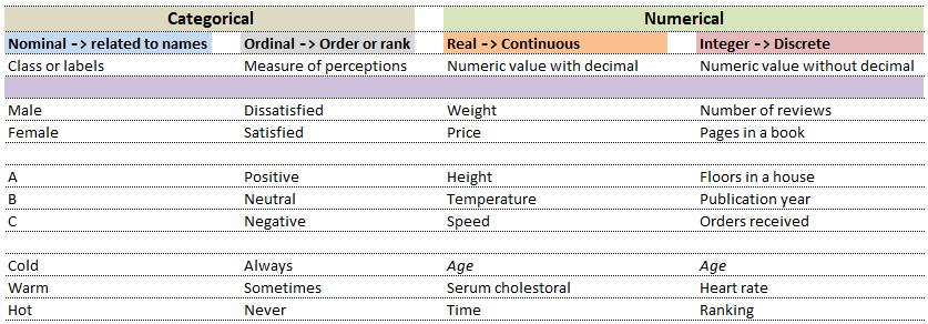
Computers understand data in a certain format whereas the nature of data can be numbers as well as words or phrases which cannot be quantified. For example, the difference in "positive and neutral" ratings cannot be quantified and will not be same as difference in "neutral and negative" ratings. There are many ways to describe the type of data we encounter in daily life such as (binary: either 0 or 1), ordered list (e.g. roll number or grade)...
| Nominal | Ordinal | ||
| What is your preferred mode of travel? | How will you rate our services? | ||
| 1 | Flights | 1 | Satisfied |
| 2 | Trains | 2 | Neutral |
| 3 | Drive | 3 | Dissatisfied |
While in the first case, digits 1, 2 and 3 are just variable labels [nominal scale] whereas in the second example, the same numbers (digits) indicate an order [ordinal scale]. Similarly, phone numbers and pin (zip) codes are 'numbers' but they form categorical variables as no mathematical operations normally performed on 'numbers' are applicable to them.

Data Analytics, Data Science, Machine Learning, Artificial Intelligence, Neural Network and Deep Learning are some of the specialized applications dealing with data. There is no well-defined boundaries as they necessarily overlap and the technology itself is evolving at rapid pace. Among these themes, Artificial Neural Network (ANN) is a technology inspired by neurons in human brains and ANN is the technology behind artificial intelligence where attempts are being made to copy how human brain works. 'Data' in itself may not have 'desired' or 'expected' value and the user of the data need to find 'features' to make machine learning algorithms works as most of them expect numerical feature vectors with a fixed size. This is also known as "feature engineering".
- Artificial Intelligence (AI): Self-driving car (autonomous vehicles), speech recognition
- Machine Learning (ML): Given a picture - identify steering angle of a car, Google translate, Face recognition, Identify hand-written letters.
| Artificial Intelligence | Machine Learning | Deep Learning |
| Engineer | Researcher | Scientist |
| B. Tech. degree | Master's degree | PhD |
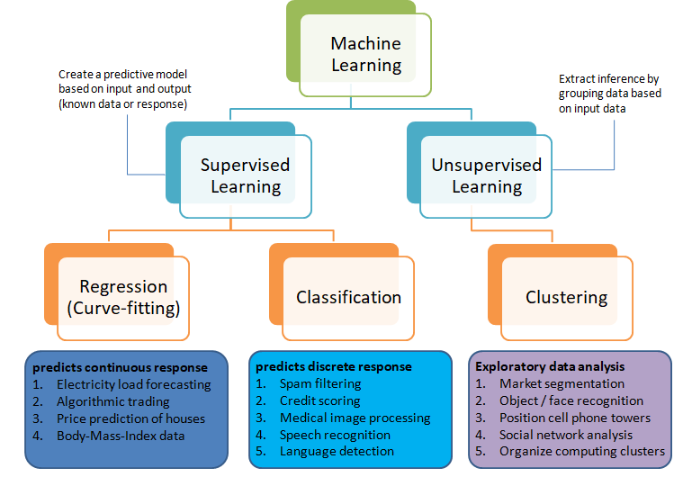
The category of supervised and unsupervised learning can be demonstrated as per the chart below. The example applications of each type of the machine learning method helps find a clear distinction among those methods. The methods are nothing new and we do it very often in our daily life. For example, ratings in terms of [poor, average, good, excellent] or [hot, warm, cold] or [below expectations, meets expectations, exceeds expectations, substantially exceeds expectations] can be based on different numerical values. Refer the customer loyalty rating (also known as Net Promoters Score) where a rating below 7 on scale of 10 is considered 'detractors', score between '7 - 8' is rated 'passive' and score only above 8 is considered 'promoter'. This highlights the fact that no uniform scale is needed for classifications.
Selection of machine learning algorithms: reference e-book "Introducing Machine Learning" by MathWorks.
Machine learning is all about data and data is all about row and column vectors. Each instance of a data or observation is usually represented by a row vector where the first or the last element may be the 'variable or category desired to be predicted'. Thus, there are two broad division of a data set: features and labels (as well as levels of the labels).
- Features: This refers to key characteristics of a dataset or entity. In other words, features are properties that describe each instance of data. Each instance is a point in feature space. For example, a car may have color, type (compact, sedan, SUV), drive-type (AWD, 4WD, FWD, RWD) ... This is also known as predictors, inputs or attributes.
- Label: This is the final identifier such as price category of a car. It is also known as the target, response or output of a feature vector.
As in any textbook, there are solved examples to demonstrate the theory explained in words, equations and figures. And then there are examples (with or without known answers) to readers to solve and check their learnings. The two sets of question can be classified as "training questions" and "evaluation questions" respectively. Similarly in machine learning, we may have a group of datasets where output or label is known and another datasets where labels may not be known.
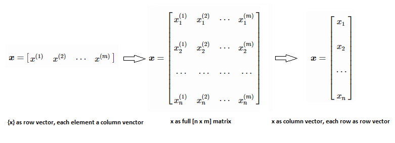
Training set is an input data where for every predefined set of features 'xi' we have a correct classification y. It is represented as tuples [(x1, y1), (x2, y2), (x3, y3) ... (xk, yk)] which represents 'k' rows in the dataset. Rows of 'x' correspond to observations and columns correspond to variables or attributes or labels. In other words, feature vector 'x' can be represented in matrix notation as: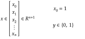
Hypothesis (the Machine Learning Model)
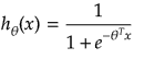
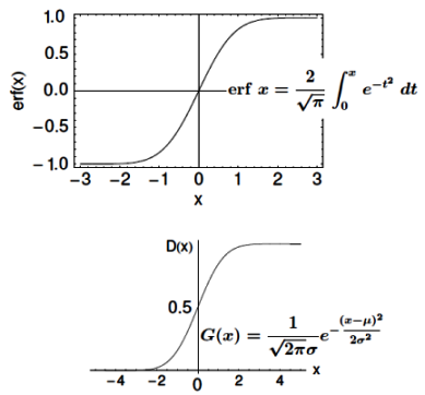
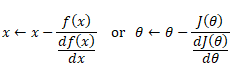
It is equation that gets features and parameters as an input and predicts the value as an output (i.e. predict if the email is spam or not based on some email characteristics). hθ(x) = g(θTx) where 'T' refers to transpose operation, θ are the (unknown) parameters evaluated during the learning process and 'g' is the Sigmoid function g(u) = [1+e-u]-1 which is plotted below.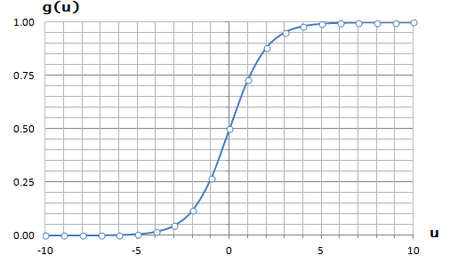
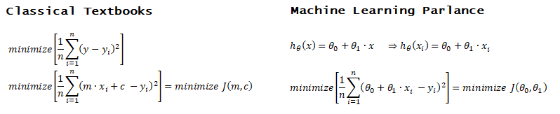
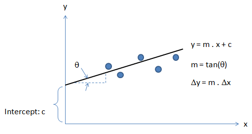
Activation Function: The hypothesis for a linear regression can be in the form y = m·x + c or y = a + b·log(c·x). The objective function is to estimate value of 'm' and 'c' by minimizing the square error as described in cost function.
The objective function of a logistic regression can be described as:- Predict y = 0 if hθ(x) < 0.5 which is true if θTx ≥ 0.
- Predict y = 1 if hθ(x) > 0.5 which is true if θTx < 0. θi are called parameters of the model.
Note that the Sigmoid function looks similar to classical error function and cumulative normal distribution function with mean zero.
Surrogate Models
These are simplified analytical models that mimic the input/output behaviour of complex systems. Developing such models requires performing computationally expensive simulations at a set of carefully selected sample points. These models approximate the behaviour of the underlying complex simulations to a reasonable precision while also being computationally cheaper to evaluate. Surrogate models are of particular interest where expensive simulations are used or when the fundamental relationship between the design variables and output variables is not well understood.Machine Learning Methods
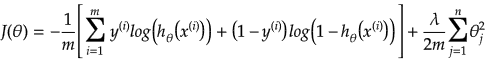
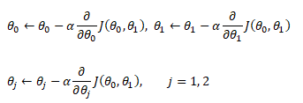
Linear regression: cost function also known as "square error function" is expressed as
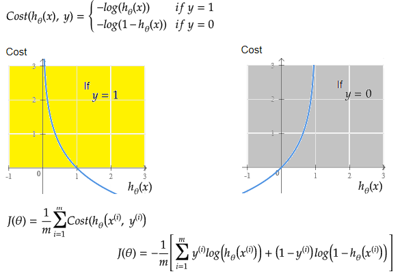
Cost(θ) = - y × log[hθ(x)] - (1-y) × [1 - log(hθ(x))]
In other words: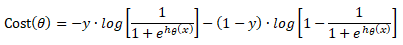
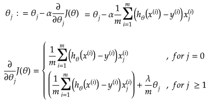
Additional method adopted is the "mean normalization" where all the features are displacement such that their means are closer to 0. These two scaling of the features make the gradient descent method faster and ensures convergence.
Normal Equation
This refers to the analytical method to solver for θ. If the matrix XTX is invertible, θ = (XTX)-1XTy where y is column vector of known labels (n × 1). X is features matrix of size n × (m+1) having 'n' number of datasets (rows) in training set and 'm' number of attributes.If [X] contains any redundant feature (a feature which is dependent on other features), it is likely to be XTX non-invertible.
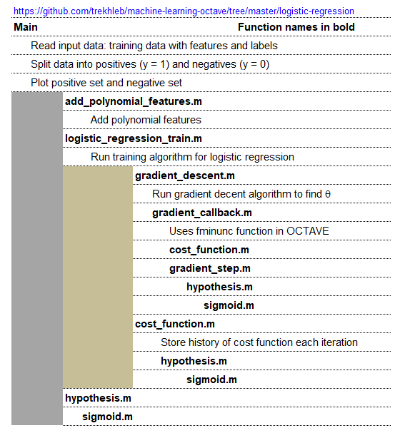
An implementation of logistic regression in OCTAVE is available on the web. One of these available in GitHub follow the structure shown below.
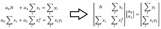
Optimization and regression using Octave - click to get the GNU OCTAVE scripts. Linear Least Square (LSS) is a way to estimate the curve-fit parameters. A linear regression is fitting a straight line y = a0 + a1x where {x} is the independent variable and y is the dependent variable. Since there are two unknowns a0 and a1, we need two equations to solve for them. If there are N data points:
Similarly, if dependent variable y is function of more than 1 independent variables, it is called multi-variable linear regression where y = f(x1, x2...xn). The curve fit equations is written as y = a0 + a1x1 + a2x2 + ... + anxn + ε where ε is the curve-fit error. Here xp can be any higher order value of xjk and/or interaction term (xi xj).
Following Python script performs linear regression and plots the discrete data, linear equation from curve-fitting operation and annotates the linear equation on the plot.
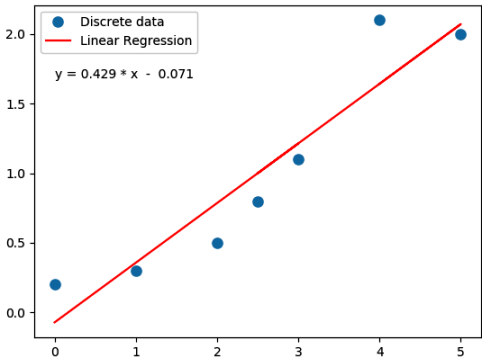
import numpy as np
#Specify coefficient matrix: independent variable values
x = np.array([0.0, 1.0, 2.0, 3.0, 2.5, 5.0, 4.0])

#Specify ordinate or "dependent variable" values
y = np.array([0.2, 0.3, 0.5, 1.1, 0.8, 2.0, 2.1])

#Create coefficient matrix
A = np.vstack([x, np.ones(len(x))]).T

#least square regression: rcond = cut-off ratio for small singular values of a
#Solves the equation [A]{x} = {b} by computing a vector x that minimizes the
#squared Euclidean 2-norm | b - {A}.{x}|^2
m, c = np.linalg.lstsq(A, y, rcond=None)[0]

print("\n Slope = {0:8.3f}".format(m))
print("\n Intercept = {0:8.3f}".format(c))

import matplotlib.pyplot as plt
_ = plt.plot(x, y, 'o', label='Discrete data', markersize=8)
_ = plt.plot(x, m*x + c, 'r', label='Linear Regression')
_ = plt.legend()
if (c > 0):
    eqn = "y ="+str("{0:6.3f}".format(m))+' * x  + '+str("{0:6.3f}".format(c))
else:
    eqn = "y ="+str("{0:6.3f}".format(m))+' * x  - '+str("{0:6.3f}".format(abs(c)))

print('\n', eqn)
#Write equation on the plot
# text is right-aligned
plt.text(min(x)*1.2, max(y)*0.8, eqn, horizontalalignment='left')
plt.show()
If the equation used to fit has exponent of x > 1, it is called a polynomical regression. A quadratic regression uses polynomial of degree 2 (y = a0 + a1x + a2x2 + ε), a cubic regression uses polynomial of degree 3 (y = a0 + a1x + a2x2 + a3x3 + ε) and so on. Since the coefficients are constant, a polynomial regression in one variable can be deemed a multi-variable linear regression where x1 = x, x2 = x2, x3 = x3 ... In scikit-learn, PolynomialFeatures(degree = N, interaction_only = False, include_bias = True, order = 'C') generates a new feature matrix consisting of all polynomial combinations of the features with degree less than or equal to the specified degree 'N'. E.g. poly = PolynomialFeatures(degree=2), Xp = poly.fit_transform(X, y) will transform [x1, x2] to [1, x1, x2, x1*x1, x1*x2, x2*x2]. Argument option "interaction_only = True" can be used to create only the interaction terms. Bias column (added as first column) is the feature in which all polynomial powers are zero (i.e. a column of ones - acts as an intercept term in a linear model).
Polynomial regression in single variable - Uni-Variate Polynomial Regression: The Polynomial Regression can be perform using two different methods: the normal equation and gradient descent. The normal equation method uses the closed form solution to linear regression and requires matrix inversion which may not require iterative computations or feature scaling. Gradient descent is an iterative approach that increments theta according to the direction of the gradient (slope) of the cost function and requires initial guess as well.
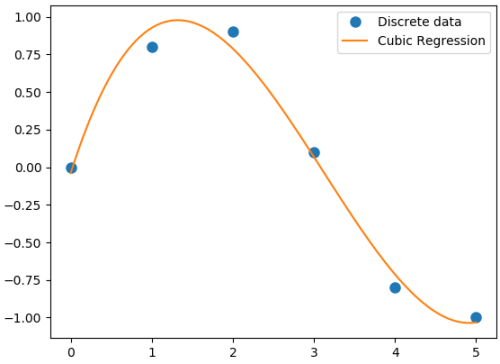
#Least squares polynomial fit: N = degree of the polynomial

#Returns a vector of coefficients that minimises the squared error in the order
#N, N-1, N-2 … 0. Thus, the last coefficient is the constant term, and the first
#coefficient is the multiplier to the highest degree term, x^N

import warnings; import numpy as np
x = np.array([0.0, 1.0, 2.0, 3.0,  4.0,  5.0])
y = np.array([0.0, 0.8, 0.9, 0.1, -0.8, -1.0])
#
N = 3
#full=True: diagnostic information from SVD is also returned
coeff = np.polyfit(x, y, N, rcond=None, full=True, w=None, cov=False)

np.set_printoptions(formatter={'float': '{: 8.4f}'.format})
print("Coefficients: ", coeff[0])
print("Residuals:", coeff[1])
print("Rank:", coeff[2])
print("Singular Values:", coeff[3])
print("Condition number of the fit: {0:8.2e}".format(coeff[4]))

#poly1D: A 1D polynomial class  e.g. p = np.poly1d([3, 5, 8]) = 3x^2 + 5x + 8
p = np.poly1d(coeff[0])

xp = np.linspace(x.min(), x.max(),100)
import matplotlib.pyplot as plt
_ = plt.plot(x, y, 'o', label='Discrete data', markersize=8)
_ = plt.plot(xp, p(xp), '-', label='Cubic Regression', markevery=10)
_ = plt.legend()

plt.rcParams['path.simplify'] = True
plt.rcParams['path.simplify_threshold'] = 0.0
plt.show()
Output from the above code is:
Coefficients:  [0.0870  -0.8135   1.6931  -0.0397]
Residuals: [ 0.0397]
Rank: 4
Singular Values: [1.8829   0.6471   0.1878   0.0271]
Condition number of the fit: 1.33e-15
In addition to 'poly1d' to estimate a polynomial, 'polyval' and 'polyvalm' can be used to evaluate a polynomial at a given x and in the matrix sense respectively. ppval(pp, xi) evaluate the piecewise polynomial structure 'pp' at the points 'xi' where 'pp' can be thought as short form of piecewise polynomial.
Similarly, a non-linear regression in exponential functions such as y = c × ekx can be converted into a linear regression with semi-log transformation such as ln(y) = ln(c) + k.x. It is called semi-log transformation as log function is effectively applied only to dependent variable. A non-linear regression in power functions such as y = c × xk can be converted into a linear regression with log-log transformation such as ln(y) = ln(c) + k.ln(x). It is called log-log transformation as log function is applied to both the independent and dependent variables.
A general second order model is expressed as described below. Note the variable 'k' has different meaning as compared to the one described in previous paragraph. Here k is total number of independent variables and n is number of rows (data in the dataset).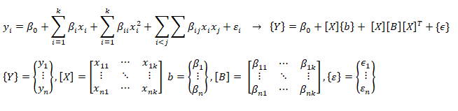
As per MathWorks: "The multivariate linear regression model is distinct from the multiple linear regression model, which models a univariate continuous response as a linear combination of exogenous terms plus an independent and identically distributed error term." Note that endogenous and exogenous variables are similar but not same as dependent and independent variables. For example, the curve fit coefficients of a linear regression are variable (since they are based on x and y), they are called endogenous variables - values that are determined by other variables in the system. An exogenous variable is a variable that is not affected by other variables in the system. In contrast, an endogenous variable is one that is influenced by other factors in the system. Here the 'system' may refer to the "regression algorithm".
In summary, categorization of regression types:
#----------------------- -------------------------- ---------------------------
import numpy as np
import pandas as pd

df = pd.read_csv('MultiVariate2.csv', sep=',', header='infer')
X = df.values[0:20, 0:3]
y = df.values[0:20, 3]

#Y = a1x1 + a2x2 + a3x3 + ... + +aNxN + c

#-------- Method-1: linalg.lstsq ---------------------- -----------------------
X = np.c_[X, np.ones(X.shape[0])] # add bias term
beta_hat = np.linalg.lstsq(X, y, rcond=None)[0]
print(beta_hat)

print("\n------ Runnning Stats Model ----------------- --------\n")
#Ordinary Least Squares (OLS), Install: py -m pip -U statsmodels
from statsmodels.api import OLS
model = OLS(y, X)
result = model.fit()
print (result.summary())

#-------- Method-3: linalg.lstsq ----------------------- ----------------------
print("\n-------Runnning Linear Regression in sklearn ---------\n")
from sklearn.linear_model import LinearRegression
regressor = LinearRegression()
regressor.fit(X, y)
print(regressor.coef_)       #print curve-fit coefficients
print(regressor.intercept_)  #print intercept values
#
#print regression accuracy: coefficient of determination R^2 = (1 - u/v), where
#u is the residual sum of squares and v is the total sum of squares.
print(regressor.score(X, y))
#
#calculate y at given x_i
print(regressor.predict(np.array([[3, 5]])))
More example of curve-fit using SciPy
'''
Curve fit in more than 1 independent variables.
Ref: stackoverflow.com/.../fitting-multivariate-curve-fit-in-python
'''
import numpy as np
import matplotlib.pyplot as plt
from scipy.optimize import curve_fit

def fit_circle(x, a, b):
  '''
  Model Function that provides the type of fit y = f(x). It must take
  the independent variable as the first argument and the parameters
  to fit as separate remaining arguments.
  '''
  return  a*x[0]*x[0] + b*x[1]*x[1]

def fit_poly(x, a, b, c, d, e, f):
  '''
  Model Function that provides the type of fit y = f(x). It must take
  the independent variable as the first argument and the parameters
  to fit as separate remaining arguments.
  '''
  return  a*x[0]*x[0] + b*x[1]*x[1] + c*x[0]*x[1] + d * x[0] + e * x[1] + f

def fit_lin_cross(x, a, b, c, d):
  '''
  Model Function that provides the type of fit y = f(x). It must take
  the independent variable as the first argument and the parameters
  to fit as separate remaining arguments.
  '''
  return a*x[0] + b*x[1] + c*x[0]*x[1] + d

def fit_2d_data(fit_func, x_data, y_data, p0=None):
  '''
  Main function to calculate coefficients.
  x_data: (k,M)-shaped array for functions with k predictors (data points)
  y_data: The dependent data, a length M array
  p0: Initial guess for the parameters (length N), default = 1
  '''
  fitParams, fitCovariances = curve_fit(fit_func, x_data, y_data, p0)

  print('Curve-fit coefficients: \n', fitParams)

# Run curve-fit. x, y and z arrays can be read from a text file.
x = np.array([1, 2, 3, 4, 5, 6])
y = np.array([2, 3, 4, 5, 6, 8])
z = np.array([5, 13, 25, 41, 61, 100])
x_data = (x, y)
fit_2d_data(fit_lin_cross, x_data, z)
Ridge Regression
If data suffers from multicollinearity (independent variables are highly correlated), the least squares estimates result in large variances which deviates the observed value far from the true value (low R-squared, R2). By adding a degree of bias to the regression estimates using a "regularization or shrinkage parameter", ridge regression reduces the standard errors. In scikit-learn, it is invoked by "from sklearn.linear_model import Ridge". The function is used by: reg = Ridge(alpha=0.1, fit_intercept=True, normalize=False, solver='auto', random_state=None); reg.fit(X_trn, y_trn). Regularization improves the conditioning of the problem and reduces the variance of the estimates. Larger values specify stronger regularization.
Lasso Regression
Lasso (Least Absolute Shrinkage and Selection Operator) is similar to ridge regression which penalizes the absolute size of the regression coefficients instead of squares in the later. Thus, ridge regression uses L2-regularization whereas as LASSO use L1-regularization. In scikit-learn, it is invoked by "from sklearn.linear_model import Lasso". The function is used by: reg = Lasso(); reg.fit(X_trn, y_trn)SVR
Support Vector Machines (SVM) used for classification can be extended to solve regression problems and method is called Support Vector Regression (SVR).Regression in two variables: example
| X1 | X2 | y | X1 | X2 | y | X1 | X2 | y | X1 | X2 | y | |||
| 5 | 20 | 100.0 | First Interpolation on X2 | Second Interpolation on X2 | Final interpolation on X1 | |||||||||
| 10 | 20 | 120.0 | 5 | 20 | 100.0 | 10 | 20 | 120.0 | 5 | 25 | 200.0 | |||
| 5 | 40 | 500.0 | 5 | 40 | 500.0 | 10 | 40 | 750.0 | 10 | 25 | 277.5 | |||
| 10 | 40 | 750.0 | ||||||||||||
| 8 | 25 | ? | 5 | 25 | 200.0 | 10 | 25 | 277.5 | 8 | 25 | 246.5 | |||
Interpolate your values:
| Description | Xi1 | Xi2 | yi |
| First set: | |||
| Second set: | |||
| Third set: | |||
| Fourth set: | |||
| Desired interpolation point: | |||
from sklearn.preprocessing import PolynomialFeatures
from sklearn.linear_model import LinearRegression
from sklearn import linear_model
import numpy as np
import pandas as pd
import sys
#Degree of polynomial: note N = 1 implies linear regression
N = 3;
#--------------- DATA SET-1 -------------------- ------------------- -----------
X = np.array([[0.4, 0.6, 0.8], [0.5, 0.3, 0.2], [0.2, 0.9, 0.7]])
y = [10.1, 20.2, 15.5]
print(np.c_[X, y]) # Column based concatenation of X and y arrays

#-------------- DATA SET-2 -------------- ------------------- ------------------
# Function importing Dataset
df = pd.read_csv('Data.csv', sep=',', header='infer')
#Get size of the dataframe. Note that it excludes header rows
iR, iC = df.shape

# Feature matrix
nCol = 5   #Specify if not all columns of input dataset to be considered
X = df.values[:, 0:nCol]
y = df.values[:, iC-1]
print(df.columns.values[0]) #Get names of the features

#Print header: check difference between df.iloc[[0]], df.iloc[0], df.iloc[[0,1]]
#print("Header row\n", df.iloc[0])

p_reg = PolynomialFeatures(degree = N, interaction_only=False, include_bias=False)
X_poly = p_reg.fit_transform(X)
#X will transformed from [x1, x2] to [1, x1, x2, x1*x1, x1x2, x2*x2]
X_poly = p_reg.fit_transform(X)

#One may remove specific polynomial orders, e.g. 'x' component
#Xp = np.delete(Xp, (1), axis = 1)

#Generate the regression object
lin_reg = LinearRegression()

#Perform the actual regression operation: 'fit'
reg_model = lin_reg.fit(X_poly, y)

#Calculate the accuracy
np.set_printoptions(formatter={'float': '{: 6.3e}'.format})
reg_score = reg_model.score(X_poly, y)
print("\nRegression Accuracy = {0:6.2f}".format(reg_score))
#reg_model.coef_[0] corresponds to 'feature-1', reg_model.coef_[1] corresponds
#to 'feature2' and so on. Total number of coeff = 1 + N x m + mC2 + mC3 ...
print("\nRegression Coefficients =", reg_model.coef_)
print("\nRegression Intercepts = {0:6.2f}".format(reg_model.intercept_))
#
from sklearn.metrics import mean_squared_error, r2_score
# Print the mean squared error (MSE)
print("MSE: %.4f" % mean_squared_error(y, reg_model.predict(X_poly)))
# Explained variance score (R2-squared): 1.0 is perfect prediction
print('Variance score: %.4f' % r2_score(y, reg_model.predict(X_poly)))
#
#xTst is set of independent variable to be used for prediction after regression
#Note np.array([0.3, 0.5, 0.9]) will result in error. Note [[ ... ]] is required
#xTst = np.array([[0.2, 0.5]])

#Get the order of feature variables after polynomial transformation
from sklearn.pipeline import make_pipeline
model = make_pipeline(p_reg, lin_reg)
print(model.steps[0][1].get_feature_names())

#Print predicted and actual results for every 'tD' row
np.set_printoptions(formatter={'float': '{: 6.3f}'.format})
tD = 3
for i in range(1, round(iR/tD)):
    tR = i*tD
    xTst = [df.values[tR, 0:nCol]]
    xTst_poly = p_reg.fit_transform(xTst)
    y_pred = reg_model.predict(xTst_poly)
    print("Prediction = ", y_pred, " actual = {0:6.3f}".format(df.values[tR, iC-1]))
For all regression activities, statistical analysis is a necessity to determine the quality of the fit (how well the regression model fits the data) and the stability of the model (the level of dependence of the model parameters on the particular set of data). The appropriate indicators for such studies are the residual plot (for quality of the fit) and 95% confidence intervals (for stability of the model).
A web-based application for "Multivariate Polynomial Regression (MPR) for Response Surface Analysis" can be found at www.taylorfit-rsa.com. A dataset to test a multivariable regression model is available at UCI Machine Learning Repository contributed by I-Cheng Yeh, "Modeling of strength of high performance concrete using artificial neural networks", Cement and Concrete Research, Vol. 28, No. 12, pp. 1797-1808 (1998). The actual concrete compressive strength [MPa] for a given mixture under a specific age [days] was determined from laboratory. Data is in raw form (not scaled) having 1030 observations with 8 input variables and 1 output variable.
In general, it is difficult to visualize plots beyond three-dimension. However, the relation between output and two variables at a time can be visualized using 3D plot functionality available both in OCTAVE and MATPLOTLIB.
Getting the training data: The evaluation of machine learning algorithm requires set of authentic data where the inputs and labels are correctly specified. However, 'make_blobs' module in scikit-learn is a way to generate (pseudo)random dataset which can be further used to train the ML algorithm. Following piece of code available from jakevdp.github.io/PythonDataScienceHandbook/05.12-gaussian-mixtures.html: Python Data Science Handbook by Jake VanderPlas is a great way to start with.
import matplotlib.pyplot as plt
from sklearn.datasets.samples_generator import make_blobs
X, y = make_blobs(n_samples=400, centers=4, cluster_std=0.60, random_state=0)
X = X[:, ::-1]  # flip axes for better plotting
plt.scatter(X[:, 0], X[:, 1], c=y, s=40, cmap='viridis', zorder=2)
plt.axis('equal')
plt.show()
This generates a dataset as shown below. Note that the spread of data points can be controlled by value of argument cluster_std. 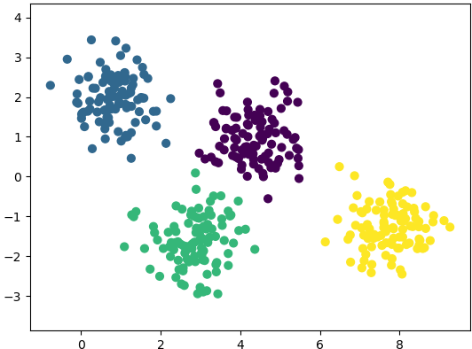
In regression, output variable requires input variable to be continuous in nature. In classifications, output variables require class label and discrete input values.
Under-fitting:
The model is so simple that it cannot represent all the key characteristics of the dataset. In other words, under-fitting is when the model had the opportunity to learn something but it didn't. It is said to have high bias and low variance. The confirmation can come from "high training error" and "high test error" values. In regression, fitting a straight line in otherwise parabolic variation of the data is under-fitting. Thus, adding a higher degree feature is one of the ways to reduce under-fitting. 'Bias' refers to a tendency towards something. e.g. a manager can be deemed biased if he continuously rates same employee high for many years though it may be fair and the employee could have been outperforming his colleagues. Similarly, a learning algorithm may be biased towards a feature and may 'classify' an input dataset to particular 'type' repeatedly. Variance is nothing but spread. As known in statistics, standard deviation is square root of variance. Thus, a high variance refers to the larger scattering of output as compared to mean.Over-fitting:
The model is so detailed that it represents also those characteristics of the dataset which otherwise would have been assumed irrelevant or noise. In terms of human learning, it refers to memorizing answers to questions without understanding them. It is said to have low bias and high variance. The confirmation can come from "very low training error - near perfect behaviour" and "high test error" values. Using the example of curve-fitting (regression), fitting a parabolic curve in otherwise linearly varying data is over-fitting. Thus, reducing the degree feature is one of the ways to reduce over-fitting. Sometime, over-fitting is also described is "too good to be true". That is the model fits so well that in cannot be true.
| ML Performance | If number of features increase | If number of parameters increase | If number of training examples increase |
| Bias | Decreases | Decreases | Remains constant |
| Variance | Increases | Increases | Decreases |
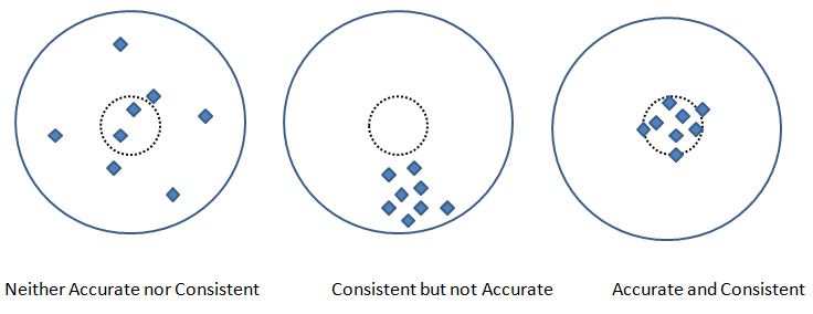
Precision and Recall are two other metric used to check the fidelity of the model. In measurements, 'accuracy' refers to the closeness of a measured value to a standard or known value and 'precision' refers to the closeness of two or more measurements to each other. Precision is sometimes also referred as consistency. Following graphics explains the different between accuracy and precision or consistency.
Pickling
Run the program of learning or training the datasets once and use its parameters every time the code is run again - this process is called pickling (analogous to classical pickles we eat)! In scikit-learn, save the classifier to disk (after training):
from sklearn.externals import joblibjoblib.dump(clf, 'pickledData.pkl')
Load the pickled classifierclf = joblib.load('pickledDatae.pkl')
It is the process of reducing the number of attributes or labels or random variables by obtaining a set of 'unique' or "linearly independent" or "most relevant" or 'principal' variables. For example, if length, width and area are used as 'label' to describe a house, the area can be a redundant variable which equals length × width. The technique involves two steps: [1]Feature identification/selection and [2]Feature extraction. The dimensionality reduction can also be accomplished by finding a smaller set of new variables, each being a combination of the input variables, containing essentially the same information as the input variables. For example, a cylinder under few circumstances can be represented just by a disk where its third dimension, height or length of the cylinder is assumed to be of less important. Similarly, a cube (higher dimensional data) can be represented by a square (lower dimensional data).
- Principal Component Analysis (PCA): This method dates back to Karl Pearson in 1901, is an unsupervised algorithm that creates linear combinations of the original features. The new features are orthogonal, which means that they are linearly independent or uncorrelated. PCA projects the original samples to a low dimensional subspace, which is generated by the eigen-vectors corresponding to the largest eigen-values of the covariance matrix of all training samples. PCA aims at minimizing the mean-squared-error. [Reference: A survey of dimensionality reduction techniques C.O.S. Sorzano, J. Vargas, A. Pascual-Montano] - The key idea is to find a new coordinate system in which the input data can be expressed with many less variables without a significant error.
- Linear Discriminant Analysis (LDA): A "discriminant function analysis" is used to determine which variables discriminate (differentiate or distinguish) between two or more groups or datasets (it is used as either a hypothesis testing or exploratory method). Thus, LDA like PCA, also creates linear combinations of input features. However, LDA maximizes the separability between classes whereas PCA maximizes "explained variance". The analysis requires the data to have appropriate class labels. It is not suitable for non linear dataset.
- Generalized Discriminant Analysis (GDA): The GDA is a method designed for non-linear classification based on a kernel function φ which transform the original space X to a new high-dimensional (linear) feature space. In cases where GDA is used for dimensionality reduction techniques, GDA projects a data matrix from a high-dimensional space into a low-dimensional space by maximizing the ratio of "between-class scatter" to "within-class scatter".
Principal Component Analysis - PCA in OCTAVE
%                                PCA
%PCA: Principal component analysis using OCTAVE -  principal components similar
%to principal stress and strain in Solid Mechanics, represent the directions of
%the data that contains  maximal amount of variance. In  other words, these are
%the lines (in 2D) and planes in (3D) that capture most information of the data.
%Principal components  are less interpretable and may not have any real meaning
%since they are constructed as linear combinations of the initial variables.
%
%Few references:
%https://www.bytefish.de/blog/pca_lda_with_gnu_octave/
%Video on YouTube by Andrew NG
%
 clc; clf; hold off;

% STEP-1: Get the raw data, for demonstration sake random numbers are used

%Generate an artificial data set of n x m = iR x iC size
 iR = 11;  % Total number of rows or data items or training examples
 iC = 2;   % Total number of features or attributes or variables or dimensions
 k  = 2;   % Number of principal components to be retained out of n-dimensions

 X = [2 3; 3 4; 4 5; 5 6; 5 7; 2 1; 3 2; 4 2; 4 3; 6 4; 7 6];
 Y = [  1;   2;   1;   2;   1;   2;   2;   2;   1;   2;   2];
 c1 = X(find(Y == 1), :);
 c2 = X(find(Y == 2), :);
 hold on;
 subplot(211);  plot(X(:, 1), X(:, 2), "ko", "markersize", 8, "linewidth", 2);
 xlim([0 10]); ylim([0 10]);
%
% STEP-2: Mean normalization

% mean(X, 1): MEAN of columns - a row vector {1 x iC}
% mean(X, 2): MEAN of rows - a column vector of size {iR x 1}
% mean(X, n): MEAN of  n-th dimension
  mu = mean(X);

% Mean normalization and/or standardization
  X1 = X - mu;
  Xm = bsxfun(@minus, X, mu);
% Standardization
  SD = std(X);     %SD is a row vector - stores STD. DEV. of each column of [X]
  W = X - mu / SD;

% STEP-3: Linear Algebra - Calculate eigen-vectors and eigen-values
% Method-1: SVD function
% Calculate eigenvectors and eigenvalues of the covariance matrix. Eigenvectors
% are unit vectors and orthogonal, therefore the norm is one and inner (scalar,
% dot) product is zero. Eigen-vectors are direction of principal components and
% eigen-values are value of variance associated with each of these components.

  SIGMA = (1/(iC-1)) * X1 * X1';  % a [iR x iR] matrix
% SIGMA == cov(X')

% Compute singular value decomposition of SIGMA where SIGMA = U*S*V'
  [U, S, V] = svd(SIGMA);   % U is iR x iR matrix, sorted in descending order
% Calculate the data set in the new coordinate system.
  Ur = U(:, 1:k);
  format short G;
  Z = Ur' * X1;
  round(Z .* 1000) ./ 1000;
%
% Method-2: EIG function
% Covariance matrix is a symmetric square matrix having variance values on the
% diagonal and covariance values off the diagonal. If X is n x m then cov(X) is
% m x m matrix. It is actually the sign of the covariance that matters :
% if positive, the two variables increase or decrease together (correlated).
% if negative, One increases when the other decreases (inversely correlated).

% Compute right eigenvectors V and eigen-values [lambda]. Eigenvalues represent
% distribution of the variance among each of the eigenvectors. Eigen-vectors in
% OCTAVE are sorted ascending, so last column is the first principal component.
  [V, lambda] = eig(cov(Xm));  %solve for (cov(Xm) - lambda x [I]) = 0

% Sort eigen-vectors in descending order
  [lambda, i] = sort(diag(lambda), 'descend');
  V = V(:, i);
  D = diag(lambda);

  %P = V' * X;    % P == Z
  round(V .* 1000) ./ 1000;
%
% STEP-4: Calculate data along principal axis
% Calculate the data set in the new coordinate system, project on PC1 = (V:,1)
  x = Xm * V(:,1);
% Reconstruct it and invert mean normalization step
  p = x * V(:,1)';
  p = bsxfun(@plus, p, mu);  % p = p + mu

% STEP-5: Plot new data along principal axis
  %line ([0 1], [5 10], "linestyle", "-", "color", "b");
  %This will plot a straight line between x1, y1 = [0, 5] and x2, y2 = [1, 10]

  %args = {"color", "b", "marker", "s"};
  %line([x1(:), x2(:)], [y1(:), y2(:)], args{:});
  %This will plot two curves on same plot: x1 vs. y1 and x2 vs. y2
  s = 5;
  a1 = mu(1)-s*V(1,1); a2 = mu(1)+s*V(1,1);
  b1 = mu(2)-s*V(2,1); b2 = mu(2)+s*V(2,1);
  L1 = line([a1 a2], [b1 b2]);

  a3 = mu(1)-s*V(1,2); a4 = mu(1)+s*V(1,2);
  b3 = mu(2)-s*V(2,2); b4 = mu(2)+s*V(2,2);
  L2 = line([a3 a4], [b3 b4]);
  args ={'color', [1 0 0], "linestyle", "--", "linewidth", 2};
  set(L1, args{:});  %[1 0 0] = R from [R G B]
  args ={'color', [0 1 0], "linestyle", "-.", "linewidth", 2};
  set(L2, args{:});  %[0 1 0] = G from [R G B]

  subplot(212);
  plot(p(:, 1), p(:, 2), "ko", "markersize", 8, "linewidth", 2);
  xlim([0 10]); ylim([0 10]);
  hold off;
The output from this script is shown below. The two dashed lines show 2 (= dimensions of the data set) principal components and the projection over main principal component (red line) is shown in the second plot.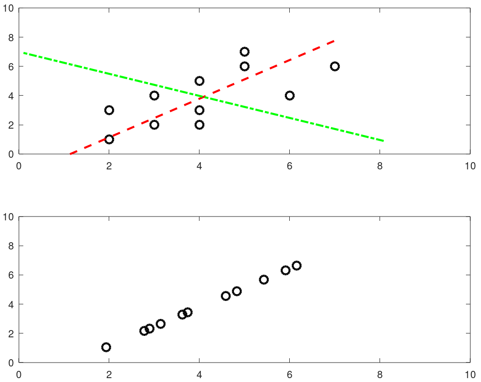
Python install / update
Install / uninstall: do not remove any older version of Python - it may uninstall Ubuntu Desktop as well. In case you unistalled a python which uninstalls Ubuntu desktop, Linux shall start in command line mode only. Use "sudo apt-get update" followed by "sudo apt-get install ubuntu-desktop" to get the desktop re-installed. It should restart with a graphical log-in prompt. If it still opens in command line mode: use 'reboot' command on the prompt. The .bash_profile shall need to be recreated especially for aliases like rm='rm -i', mv='mv -i' and cp='cp -i'.To call Python3 with just 'python' in Linux: sudo rm /usr/bin/python followed by sudo ln -s /usr/bin/python3.9 /usr/bin/python - gives error if link already exists. This way, if Python2.x is needed, it can be called explicitly with python2.x while 'python' defaults to python3 because of the symbolic link. ls -l /usr/bin/python* and ls -l /usr/local/bin/python*- get all installed versions in Linux. To make a specific version default, add in .bash_profile: alias python3='/usr/bin/python3.9'.
Install packages: sudo apt-get install python3-pip, python3 -m pip install matplotlib, pip install numpy, sudo apt-get install python3-opencv. Note that "pip install numpy" works in Linux but prints error message "Access Denied" in Windows. Use "python -m pip install numpy" in Windows terminal.OCTAVE vs. Python
You would have got a flavour of Python programming and OCTAVE script in examples provided earlier. This page does not cover about basic syntax of programming in any of the language. One thing unique in Python is the indentation. Most of the languages use braces or parentheses to define a block of code or loop and does not enforce any indentation style. Python uses indentation to define a block of statements and enforces user to follow any consistent style. For example, a tab or double spaces or triple spaces can be used for indentation but has to be only one method in any piece of code (file).
Following table gives comparison of most basic functionalities of any programming language.
| Usage | OCTAVE | Python |
| Case sensitive | Yes | Yes |
| Current working directory | pwd | import os; os.getcwd() |
| Change working directory | chdir F:\OF | import os; os.chdir("C:\\Users") |
| Clear screen | clc | import os; os.system('cls') |
| Convert number to string | num2str(123) | str(123) |
| End of statement | Semi-colon | Newline character |
| String concatenation | strcat('m = ', num2str(m), ' [kg]') | + operator: 'm = ' + str(m) + ' [kg]' |
| Expression list: tuple | - | x, y, z = 1, 2, 3 |
| Get data type | class(x) | type(x) |
| Floating points | double x | float x |
| Integers | single x | integer x, int(x) |
| User input | prompt("x = ") x = input(prompt) | print("x = ") x = input() |
| Floor of division | floor(x/y) | x // y |
| Power | x^y or x**y | x**Y |
| Remainder (modulo operator) | mod(x,y): remainder(x/y) | x%y: remainder(x/y) |
| Conditional operators | ==, <, >, != (~=), ≥, ≤ | ==, <, >, !=, ≥, ≤ |
| If Loop | if ( x == y ) x = x + 1; endif | if x == y: x = x + 1 |
| For Loop | for i=0:10 x = i * i; ... end | for i in range(1, 10): x = i * i |
| Arrays | x(5) 1-based | x[5] 0-based |
| File Embedding | File in same folder | from pyCodes import function or import pyCodes* as myFile |
| Defining a Function | function f(a, b) ... end | def f(a, b): ... |
| Anonymous (inline) Function | y = @(x) x^2; | y = lambda x : x**2 |
| Return a single random number between 0 ~ 1 | rand(1) | random.random() |
| Return a integer random number between 1 and N | randi(N) | random.randint(1,N) |
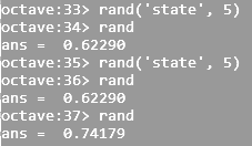
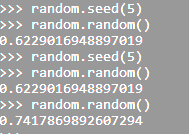
| Return a integer random number with seed | rand('state', 5) | random.seed(5) |
 |  | |
| Return a single random number between a and b | randi([5, 13], 1) | random.random(5, 13) |
| Return a (float) random number between a and b | a + (b-a)*rand(1) | random.uniform(a, b) |
| Return a (float) random number array | rand(1, N) | numpy.random.rand(N) |
| Stop execution after a statement | return | sys.exit() |
To run a function (out of many stored in a module) from the command line: $python3 -c 'import moduleName; funcName()'. The parentheses at the end of funcName makes the function be called. In Windows shell, a double quote should be used instead of single. If funcName() takes arguments, to supply by the command line use sys.argv to the method or access it from the funcName() method. Alternatively, add following lines at the end of module.
if __name__ == "__main__":
  args = sys.argv
  # args[0] = current file (module name), args[1] = function name
  # args[2:] = function args : (*unpacked)
  globals()[args[1]](*args[2:])
Here 'globals' pass the command line argument (name of the function) into locals which is a dictionary with a current local symbol table.
if __name__ == '__main__':
  moduleName()
This is the way to make the function execute (run) when the file is run and not when the file (or module) is imported.
Many use of underscore: throwaway or implicit variable such as "for _ in range(5)", stores the result of the last executed expression (_ allows to call the last function/variable), double leading and trailing underscore such as __variable__ is reserved for special methods, ignoring values such as "_, thresh = cv2.threshold(img, 127, 255, 0)", grouping thousand separator for easy readability of long literals such as 5_000_000.0
Function Annotation: -> marks the (optional) return annotation of a function and annotations are dictionaries. function_name.__annotations__ prints the details such as argument names and type, return values and type...
def func(n: float) -> int:
  return int(n)
print(func.__annotations__) gives output: "{'n': <class 'float'>, 'return': <class 'int'>}". Here the return annotation '->' infers that func() shall return an integer (though the function is not forced to return an integer). The colon separator in "n: float" specifies that 'n' should be of type float. It is like 'int' used while defining a method in (strongly typed language) Java.
public int func(float n) {
  return n * n;
}
Lambda Functions, also known as anonymous functions as they do not have name. They can have any number of arguments but can only have one expression. These are good for one task that needs repetition. Lambda functions can be used inside other regular functions. In fact, this is their main advantage. f = lambda x: x**2 #Like creating a function f, y = f(5) #Execute the function. Some other built-in functions are
zip(a, b) is equivalent to
y = []
for i in range(5):
 for j in range(3):
  if i == j:
   x = (i, j)
   y.append(x)
Ternary Operator
Python for and if on one line: find a list of items matching some criterion - [i for i in xlist if x % 2 == 1]. To find one item matching some criterion, x = next(i for i in xlist if x % 2 == 1). i = next((elm for elm in xlist if elm == 'two'), None) - i will be set to 'None' if there is no matching element. Ternary Operator: result = 'Even' if x % 2 == 0 else 'Odd'.
Tuple and Dictionary
Associative arrays used in other programming languages are called dictionaries in Python. Dictionaries are type of lists where keyrod and value pairs are stored separated by comma. E.g. dictList = {'streams': [{'index': 0, 'codec_name': 'vp9'}, {'index': 1, 'codec_type': 'audio'}], 'format': {'filename': 'in.webm', 'nb_streams': 2}} - this is a list of dictionaries named 'streams' and 'format'. The value of 'codec_type' that is 'audio' can be retrieved by codec = dictList['streams']['codec_name']. In other words, dictionaries are unordered set of key: value pairs, with the requirement that the keys are unique (within one dictionary)
From Python Documentation:- Pair of braces creates an empty dictionary: dictX = {}
- Placing a comma-separated list of key:value pairs within the braces adds initial key:value pairs to the dictionary
- keys() method of a dictionary object returns a list of all the keys used in the dictionary, in arbitrary order
- Apply the sorted() function to it keys() method to get an alphabetically sorted list: sortedKeys = sorted(dictName.keys())
- To check whether a single key is in the dictionary, use the 'in' keyword such as "x not in s" or "y in z"
- To loop through dictionaries, the key and corresponding value can be retrieved at the same time using the iteritems() method: for key, val in dictName.iteritems()
- The dict() constructor builds dictionaries directly from sequences of key-value pairs
- The .get() method retrieves the value associated with a key: keyValue = dictName.get(keyName). If the key exists, it returns the value else Boolean None is returned.
try:
  value = dictName[key]
except KeyError:
  print("Specified key is not present.\n")
  pass
An underscore is used to ignore part of a tuple returned by Python commands: _, dirnames, filenames in os.walk(path) - here the underscore simply tells that the user is not going to use first part of the three-tuple returned by os.walk. However, dpath, dname, fname = os.walk() can be used to access three-tuples returned by os.walk.
Arbitrary Positional Arguments
*args and **kwargs allow you to pass arbitrary (multiple) positional arguments and arbitrary (multiple) keyword arguments respectively to a function without declaring them beforehand. Note that keyword arguments are like dictionary with a 'key=value' pair where = is used instead of colon (:). The star (*) and double-stars (**) respectively at the start of these names are called asterisk operators or unpacking operators which return iterable objects as tuple. A tuple is similar to a list in that they both support slicing and iteration. Note that tuples are not mutable that is they cannot be changed. Tuples are specified as comma separated items inside parentheses like theTuple = (1, 2, 3) whereas lists are specified in brackets like theList = [1, 2, 3].
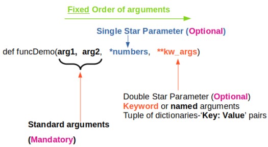
args[0] or "for arg in args" and kwargs[kwrd] or "for key, value in kwargs.items()" or "for kwval in kwargs.values()" can be used to access each members of args and kwargs lists respectively. "for key in kwargs" can be used to access 'key' names in kwargs list comprising of pairs of keywords and values.
How to check if *args[0] exists? Note that *args is a tuple (with zero, one or more elements) and it will result in a True if it contains at least one element. Thus, the presence of *args can be simply checked by "if args:" Similarly, if 'key1' in kwargs: can be used if key1 in **kwargs exists or not? len(args) ≡ args.__len__() and len(kwargs): find length of positional arguments. How to check if function is callable with given *args and **kwargs? While looping through a sequence, the position index and corresponding value can be retrieved at the same time using the enumerate() function: for idx, val in enumerate(listName)
Arrays
aRaY = [] - here aRaY refers to an empty list though this is an assignment, not a declaration. Python can refer aRaY to anything other than a list since Python is dynamically typed. The default built-in Python type is called a 'list' and not an array. It is an ordered container of arbitrary length that can hold a heterogeneous collection of objects (i.e. types do not matter). This should not be confused with the array module which offers a type closer to the C array type. However, the contents must be homogenous (all of the same type), but the length is still dynamic.This file contains some examples of array operations in NumPy.
arr = np.array( [ [0, 0, 0, 0], [0, 1, 1, 0], [0, 1, 1, 0], [0, 0, 0, 0] ] )print(arr): output is
[[0 0 0 0]
 [0 1 1 0]
 [0 1 1 0]
 [0 0 0 0]]
print(type(arr)) = <class 'numpy.ndarray'>
x = np.array([1.2, 2.3, 5.6]), x.astype(int) = array([1, 2, 6])
row_vector = array([[1, 3, 5]]) or np.r_['r', [1, 3, 5]] which has 1 row and 3 columns, col_vector = array([[2, 4, 6]]).T or np.r_['c', [2, 4, 6]] which has 3 rows and 1 column. Convert a row vector to column vector: col_vec = row_vec.reshape(row_vec.size, 1), or col_vec = row_vec.reshape(-1, 1) where -1 automatically finds the value of row_vec.size. Convert a column vector to row vector: row_vec = col_vec(1, -1). Examples:a = np.linspace(1, 5, num=5) > print(a) >> [1. 2. 3. 4. 5.] print(a.shape) >> (5,) print(a.reshape(-1, 1)) [[1.] [2.] [3.] [4.] [5.]] print((a.reshape(-1, 1)).shape) >> (5, 1) x = np.array([1,2,3,4,5]) > print(x) >> [1 2 3 4 5]. print(x.shape) >> (5,) x = np.array([[1,2,3,4,5]]) > print(x.shape) >> (1, 5) x = np.arange(1, 5, 1) > print(x) >> [1 2 3 4]. print(x.shape) >> (4,)2D operations
X = np.array([1, 2, 3]), Y = np.array([2, 4, 6]), X, Y = np.meshgrid(X, Y)
Z = (X**2 + Y**2), print(Z)
[[ 5  8 13]
 [17 20 25]
 [37 40 45]]
i.e. Z = np.array([[5, 8, 13], [17, 20, 25], [37, 40, 45]])
Summary
Python interpreter is written in C language and that array library includes array of C language. A string is array of chars in C and hence an array cannot be used to store strings such as file names.
- Floating-point arithmetic always produces a floating-point result. Hence, modulo operator for integers and floating point numbers will yield different results.
- Python uses indentation to show block structure. Indent one level to show the beginning of a block. Outdent one level to show the end of a block. The convention is to use four spaces (and not the tab character even if it is set to 4 spaces) for each level of indentation. As an example, the following C-style code:
C                       Python
if (x > 0) {            if x:
 if (y > 0)  {              if y:
        z = x+y                 z = x+y
    }                       z = x*y
    z = x*y
}
Comments: Everything after "#" on a line is ignored. Block comments starts and ends with ''' in Python. - eye(N), ones(N) and zeros(N) creates a NxN identity matrix, NxN matrix having each element '1' and NxN matrix having each element '0' respectively.
- 'seed' number in random number generators is only a mean to generate same random number again and again. This is equivalent to rng(5) in MATLAB.
- linspace(start, end, num): num = number of points. If omitted, num = 100 in MATLAB/OCTAVE and num = 50 in numpy. Note that it is number of points which is equal to (1 + number of divisions). Hence, if you want 20 divisions, set num = 21. That is, increment Δ = (end - start) / (num - 1). Available in numpy, OCTAVE/MATLAB.
- linspace(1, 20, 20) = 1:20. And hence, reshape(1:20, 4, 5) is equivalent to reshape(linspace(1, 20, 20), 4, 5)
- Arrays: use space or commas to delimit columns, use semi-colon to delimit rows. In same ways, space can be used to stack arrays column-wise (hstack in numpy) e.g. C = [A B] and semi-colon can be used to stack arrays row-wise (vstack in numpy) e.g. C = [A; B].
- In numpy, if x is a 2D array then x[0,2] = x[0][2]. NumPy arrays can be indexed with other arrays. x[np.array([3, 5, 8])] refers to the third, fifth and eighth elements of array x. Negative values can also be used which work as they do with single indices or slices. x[np.array([-3, -5, -8])] refers to third, fifth and eighth elements from the end of the vector 'x'.
- Negative indexing to call element of an array or a matrix is not allowed in OCTAVE/MATLAB. In case negative counters of a loop is present e.g. j = -n:n, use i = 1:numel(j) to access x(i).
Conditional and Logical Indexing
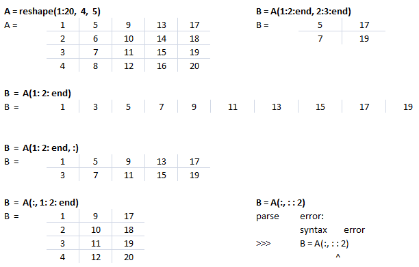
u(A < 25) = 255 replaces the elements of matrix 'u' to 255 corresponding to elements of A which is < 25. If A = reshape(1:20, 4, 5) then B = A(A>15)' will yield B = [16 17 18 19 20]. B = A; B(A < 10) = 0 will replace all those elements of matrix A which are smaller than 10 with zeros.B = A < 9 will produce a matrix B with 0 and 1 where 1 corresponds to the elements in A which meets the criteria A(i, j) < 9. Similarly C = A < 5 | A > 15 combines two logical conditions.
Find all the rows where the elements in a column 3 is greater than 10. E.g. A = reshape(1:20, 4, 5). B = A(:, 3) > 10 finds out all the rows when values in column 3 is greater than 10. C = A(B:, :) results in the desired sub-matrix of the bigger matrix A.vectorization
This refers to operation on a set of data (array) without any loop. Excerpts from OCTAVE user manual: "Vectorization is a programming technique that uses vector operations instead of element-by-element loop-based operations. To a very good first approximation, the goal in vectorization is to write code that avoids loops and uses whole-array operations". This implicit element-by-element behaviour of operations is known as broadcasting.Summation of two matrices: C = A + B
for i = 1:n
  for j = 1:m
    c(i,j) = a(i,j) + b(i,j);
  endfor
endfor
Similarly:
for i = 1:n-1
  a(i) = b(i+1) - b(i);
endfor
can be simplified as a = b(2:n) - b(1:n-1)
If x = [a b c d], x .^2 = [a2 b2 c2 d2]
The vector method to avoid the two FOR loops in above approach is: C = A + B where the program (numPy or OCTAVE) delegates this operation to an underlying implementation to loop over all the elements of the matrices appropriately.
Slicing
This refers to the method to reference or extract selected elements of a matrix or vector. Indices may be scalars, vectors, ranges, or the special operator ':', which may be used to select entire rows or columns. ':' is known as slicing object. The basic slicing syntax is "start: stop: step" where step = increment. Note that the 'stop' value is exclusive that is rows or columns will be included only up to ('stop' - 1). In NumPy (and not in OCTAVE), any of the three arguments (start, stop, step) can be omitted. Default value of 'step' = 1 and default value of 'start' is first row or column. In NumPy (not in OCTAVE) an ellipsis '...' can be used to represent one or more ':'. In other words, an Ellipsis object expands to zero or more full slice objects (':') so that the total number of dimensions in the slicing tuple matches the number of dimensions in the array. Thus, for A[8, 13, 21, 34], the slicing tuple A[3 :, ..., 8] is equivalent to A[3 :, :, :, 8] while the slicing tuple A[..., 13] is equivalent to A[:, :, :, 13]. Special slicing operation A[::-1] reverses the array A. Note that even though it is equivalent to A[len(A)-1: -1: -1], the later would produce an empty array.
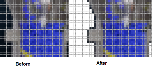
Slicing to crop an image: img_cropped = img(h0: h0+dh, w0: w0+dw) can be used to crop an image (which is stored as an array in NumPy). This one line code crops an array by number of pixels w0, h0, dw and dh from left, top, right and bottom respectively. Similarly, the part of an array (and hence an image) can be replaced with another image in this one line of code: img_source(h0: h0 + img_ref.shape[0], w0: w0 + img_ref.shape[1]) = img_ref -> here the content of image named img_ref is replaced inside img_source with top-left corner placed at w0 and h0 in width and height directions respectively.Slicing against column: B = A(3:2:end, :) will will slice rows starting third row and considering every other row thereafter until the end of the rows is reached. In numpy, B = A[:, : : 2] will slice columns starting from first column and selecting every other column thereafter. Note that the option ': : 2' as slicing index is not available in OCTAVE.
Let's create a dummy matrix A = reshape(1:20, 4, 5) and do some slicing such as B = A(:, 1:2:end). 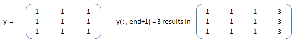

This text file contains example of Slicing in NumPy. The output for each statement has also been added for users to understand the effect of syntaxes used. There is a function defined to generate a sub-matrix of a 2D array where the remaining rows and columns are filled with 255. This can be used to crop a portion of image and filling the remaining pixels with white value, thus keeping the size of cropped image of size as the input image.
Arrays: Example syntax and comparison between OCTAVE and NumPy
| Usage | GNU OCTAVE | Python / NumPy |
| Definition | A = reshape(0:19, 4, 5)' | A = numpy.arange(20).reshape(5, 4) |
| Reshape example | 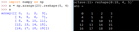 | |
| A(3) | Scalar - single element | - |
| A[3] | Not defined | Same as A[3, :]: 4th row of matrix/array |
| Special arrays | zeros(5, 8), ones(3,5,"int16") | np.zeros( (5, 8) ), np.ones( (3, 5), dtype = np.int16) |
| Create array from txt files | data = dlmread (fileName, ".", startRow, startCol) | np.genfromtxt(fileName, delimiter=",") |
3D arrays: widely used in operations on images
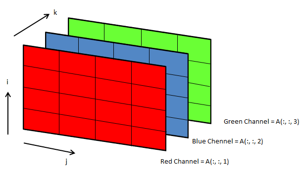
Following OCTAVE script can be used to convert the background colour of an image from black to white.
clc; clear; clear all; [x, map, alpha] = imread ("Img.png"); [nR nC nZ] = size(x);

A = x(:, :, 1); B = x(:, :, 2); C = x(:, :, 3); i = 40; u = A; v = B; w = C;
u(A<i & B<i & C<i) = 255; v(A<i & B<i & C<i) = 255; w(A<i & B<i & C<i) = 255;

z = cat(3, u, v, w); imwrite(z, "newImg.png"); imshow(z);
File Operations in Python
- List files and folders: dirpath, subdirs, files = os.walk(root_folder) - os.walk returns a three-tuple (dirpath, dirnames, filenames) where dirpath is nothing but the top-level root folder specified, subdirs = sub-directories below root folder. Thus, "for dirpath, subdirs, files in os.walk(root_folder)" will create one outer loop (list or names of sub-folders) and an inner loop (list or names of files in each sub-folder).
- As per user doc: "Note that the names in the lists contain no path components. To get a full path (which begins with top) to a file or directory in dirpath, do os.path.join(dir_path, file_name). Whether or not the lists are sorted depends on the file system."
- Sort a list: files.sort(), to list them in numeric order: sorted(files, key=int). os.walk() yields in each step what it will do in the next step(s).
- Find number of folders: n_dirs = sum([ len(dirs) for root, dirs, files in os.walk(root_folder) ])
- Number of files: n_files = sum([ len(files) for root, dirs, files in os.walk(root_folder) ])
- Check if a file exists: os.path.isfile(fileName)
- Check if a folder exists: os.path.isdir(str(dirPath))
- Get file extension: f_extn = fileName.partition('.')[-1]
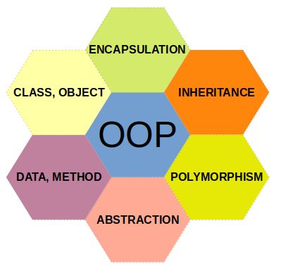
Procedural or Functional Programming vs. Object Oriented Programming - Functional programs tend to be a bit easier to follow than OOP which has intricate class hierarchies, dependencies and interactions. From learn.microsoft.com titled getting-started-with-vba-in-office: "Developers organize programming objects in a hierarchy, and that hierarchy is called the object model of the application. The definition of an object is called a class, so you might see these two terms used interchangeably. Technically, a class is the description or template that is used to create, or instantiate, an object. Once an object exists, you can manipulate it by setting its properties and calling its methods. If you think of the object as a noun, the properties are the adjectives that describe the noun and the methods are the verbs that animate the noun. Changing a property changes some quality of appearance or behavior of the object. Calling one of the object methods causes the object to perform some action."
A related concept is namespace which is a way of encapsulating items. Folders are namespace for files and other folders.
As a convention, an underscore _ at the beginning of a variable name denotes private variable in Python. Note that it is a convention as the concept of "private variables" does not exist in Python.
Class definition like function 'def' statement must be executed before used.#!/usr/bin/env python3
import math
class doMaths(): # definition of a new class
py = 3.1456 # can be accessed as doMaths.py
# Pass on arguments to a class at the time of its creation using
# __init__ function.
def __init__(self, a, b):
# Here 'self' is used to access the current instance of class, need
# not be named 'self' but has to be the first parameter of function
# Define a unique name to the arguments passed to __init__()
self.firstNum = a
self.secondNum = b
self.sqr = a*a + b* b
self.srt = math.sqrt(a*a + b*b)
print(self.sqr)
def evnNum(self, n):
if n % 2 == 0:
print(n, " is an even number \n")
else:
print(n, " is an odd number \n")
# Create an INSTANCE of the class doMaths: called Instantiate an object
xMath = doMaths(5, 8) # Output = 89
print(xMath.firstNum) # Output = 5
print(xMath.sqr) # Output = 89
# Access the method defined in the class
xMath.evnNum(8) # Output = "8 is an even number"
class doMaths(mathTricks) - here 'doMaths' class is inherited from class 'mathTricks'. When a __init__() function is added in the child class it will no long inherit the parent's __init__() function. This is called overriding the inheritance. To keep the inheritance, call parent's __init__(0 as parentClassName.__init__() such as mathTricks.__init__() in this case. Alternatively, one can use super() function. While child class (doMaths here) inherits all attributes and method definitions of parent class (mathTricks here), new attributes and methods specific to child class can be added as per the requirements. However, method with the same name and arguments in chile or derived class and parent or base or super class, the method in derived class overrides the method in the base class: this is known as Method Overriding.
Decorators: There are functions that take a function and returns some value by adding new functionalities. A decorator is assigned by adding @ before the name. Adding a decorator before a function, Python calls the function without assigning the function call to a variable. e.g.
@decore_func
def next_func():
  ...
If y = next_func() is called, next_func() ≡ y = decor_func(next_func). Multiple decorators can be chained by placing one after the other, most inner being applied first. Special decorator @property is used to define 'property' of a 'class' object. For example:
class personalData:
  ...
  @property
  def personName(self):
    return self.name
  ...
  ...
It sets personName() function as a property of a class personalData.
Python Argument Parsing
Python functions are a great way to make your code modular and granular. One can store many functions in a Python code file and pass arguments through command line using argparse module. The sample code below demonstrates how multiple functions can be called based on desired operation and arguments can be passed to each of the functions called. Either sys.argv or argparse can be used to achieve same objectives though arparse tend to be more convenient. As argparse automatically checks the presence of arguments, the conditional statements needed in sys.argv is not required with argparse. Argparse can automatically generate usage and help messages.
Excerpt from stackoverflow.com/ ~ /use-argparse-to-run-1-of-2-functions-in-my-script: If a python file is intended to be accessed in multiple ways (called as a script, loaded as a module from another python file), then the parts specific to "being run as a script" should be in your main-section. You can write a function main() and call that in a __name__ == "__main__" if block, or write your script action code directly in said if block.
Argument Parsing is a necessary step to create Command Line Interface (CLI). One can create sub-commands, add options or flags or switches using argument parsing. In example "pip install -r list.txt", install is a sub-command to main command pip, -r is an option to subcommand 'install' and list.txt is parameter to option. Note that argparse parses all arguments at once and no conditional parsing based on arguments is feasible. Alternatively, "Python Fire" is a library for automatically generating command line interfaces (CLIs) from absolutely any Python object. Fire can call a function without changing the script: python -m fire moduelName funcName. It also has a built-in argparser.
import argparse
if __name__ == "__main__":
  parser = argparse.ArgumentParser(prog='pyArgParsing',
                    description='Edit PDF Files using PyPDF2',
                    epilog='Delete, rotate and scale pages of a PDF')

  # Attach individual argument specifications to the parser: add_argument
  parser.add_argument("operation", help="Operation to be performed", \
                      choices=["delete","shuffle","scale"])
  parser.add_argument("file_name", help="Input PDF File Name")
  parser.add_argument("startPage", help="Start page number")
  parser.add_argument("endPage", help="End page number")

  # Optional arguments: '*' or '+'- All command-line arguments are gathered
  # into a list. nargs='argparse.REMAINDER': All the remaining command-line
  # arguments are gathered into a list. args='?' - does not produce a list.
  # nargs=N, N arguments from the command line collected into a list
  parser.add_argument('scale', nargs='?', default=1.0)

  args = parser.parse_args()

  if args.operation == "delete":
    deletePagesPDF(args.file_name, int(args.startPage), int(args.endPage))
  elif args.operation == "shuffle":
    shufflePagesPDF(args.file_name, int(args.startPage), int(args.endPage))
  elif args.operation == "scale":
    s=float(args.scale)
    scalePagesPDF(args.file_name, int(args.startPage), int(args.endPage), s)
Note that nargs creates a list except nargs='?'. Hence, if a function takes string as argument, such as path of a folder, do not use nargs. Else, you may get error "TypeError: stat: path should be string, bytes, os.PathLike or integer, not list". This code can be run from command line as: python3 pyArgParsing.py delete input.pdf 3 8 and python3 pyArgParsing.py scale input.pdf 3 8 1.5
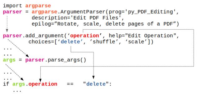
From docs.python.org/3/library/argparse.html
import argparse

parser = argparse.ArgumentParser(description='Process some integers.')
parser.add_argument('integers', metavar='N', type=int, nargs='+',
                    help='an integer for the accumulator')
parser.add_argument('--sum', dest='accumulate', action='store_const',
                    const=sum, default=max,
                    help='sum the integers (default: find the max)')

args = parser.parse_args()
print(args.accumulate(args.integers))

$- python3 testArgParser.py
usage: testArgParser.py [-h] [--sum] N [N ...]
testArgParser.py: error: the following arguments are required: N

$- python3 testArgParser.py -h
usage: testArgParser.py [-h] [--sum] N [N ...]

Process some integers.

positional arguments:
  N           an integer for the accumulator

optional arguments:
  -h, --help  show this help message and exit
  --sum       sum the integers (default: find the max)

$- python3 testArgParser.py 1 2 3 4
4

$- python3 testArgParser.py 1 2 3 4 --sum
10
Reference: docs.python.org/3/library/argparse.html
prefix_chars: Most command-line options will use hyphen - as the prefix, e.g. -name or --name. Parsers that need to support different or additional prefix characters, e.g. for options like +name or /name, may specify them using the prefix_chars= argument to the ArgumentParser constructor: parser = argparse.ArgumentParser(prog = 'denoiseImages', prefix_chars='-+'). The prefix_chars= argument defaults to '-'. Supplying a set of characters that does not include '-' will cause -name or --name options to be disallowed.There are two types of arguments: [1] positionals: these are identified by order without any identifying name and [2] optionals: these are identified by a name or flag string such as parser.add_argument("-name") or parser.add_argument("--name"). The order of optionals does not matter and optionals are similar (but not identical) to the keyword arguments of Python functions. By default, ArgumentParser groups command line arguments into "positional arguments" and 'options' displaying messages. Argument groups can be used in case such default grouping does not help.
parser.add_argument("-name"): the command line arguments should be entered as "-name Krishna". parser.add_argument("--name"): the command line arguments should be entered as "--name Krishna". In case multiple entries are made such as "-name Ram -name Krishna", the last entry shall be used by the argument parser.
parser.add_argument("-x", "--del", action="store_true"): option names start with - for shorthand flags and -- for long flags. Action argument "store_true" accompanies option indicate that this option will be stored as Boolean value. If the option at the command line is provided, its value will be True else False.
Arguments shared between parsers: There are many instances where arguments are shared across different parsers. To avoid repeating the definitions of such shared arguments, "parent=" argument to ArgumentParser can be used.
![]()
Sub-commands
Reference: docs.python.org/3.2/library/argparse.html --- Many programs split up their functionality into a number of sub-commands, a particularly good idea when a program performs several different functions which require different kinds of command-line arguments. ArgumentParser supports the creation of such sub-commands with the add_subparsers() method. The add_subparsers() method is normally called with no arguments and returns a special action object.
import argparse, sys
# Adaptation of example at docs.python.org/3/library/argparse.html#sub-commands

# Sub-command functions
def sub_cmd1(args) :
  print(args.x * args.y)

def sub_cmd2(args):
  print(args.u + args.v)

# Create the top-level parser
parser = argparse.ArgumentParser()
subparsers = parser.add_subparsers(required=True)

# Create the (sub) parser for the 'sub_cmd1' command
parser_sub_cmd1 = subparsers.add_parser('sub_cmd1')
parser_sub_cmd1.add_argument('-x', type=int, default=10)
parser_sub_cmd1.add_argument('y', type=float )
parser_sub_cmd1.set_defaults(func = sub_cmd1)

# Create the (sub) parser for the 'sub_cmd2' command
parser_sub_cmd2 = subparsers.add_parser('sub_cmd2')
parser_sub_cmd2.add_argument('-u', type=int, default=10)
parser_sub_cmd2.add_argument('v', type=int)
parser_sub_cmd2.set_defaults(func = sub_cmd2)

# Parse the arguments and call whatever function was specified on command line
if len(sys.argv) > 1:
  args = parser.parse_args()
  args.func(args)
else:
  print("\n  ---No sub-command name provided. \n")
Usage:
python3 cmd_sub.py sub_cmd1
  usage: cmd_sub.py sub_cmdi [-h] [-x X] y
  cmd sub.py sub cmd1: error: the following arguments are required: y
python3 cmd_sub.py sub_cmd1 3: output = 30.0, python3 cmd _sub.py sub_cmd1 -x 10 25: output = 250.0, python3 cmd_sub.py sub_cmd2 5: output = 15, Python3 cmd_sub.py sub_cmd2 -u 4 5: output = 9
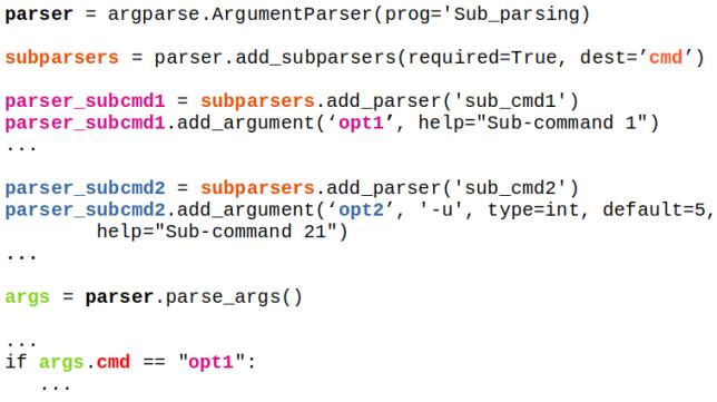
Note that the sub-commands used in above example are the names of the 'functions'. If sub-commands are intended to be a 'switch' to activate a particular loop or conditional statement of a function, following example can be used. Here, 'files' and 'folder' are mere options to be passed on to the function mergePDF().
parser = argparse.ArgumentParser()
subparsers = parser.add_subparsers(dest="command")

# Create the (sub) parser for the 'files' command
parser_files = subparsers.add_parser('files',
                                 help="Merge files specified on command line")
parser_files.add_argument('-f', nargs='*')

# Create the (sub) parser for the 'folder' command
parser_folder = subparsers.add_parser('folder',
                                 help="Merge PDF files in specified directory")
parser_folder.add_argument('-d', nargs=1)

# Parse the arguments and call whatever function was specified on command line
args = parser.parse_args()
if args.command == 'files':
  if args.f:
    mergePDF(0, args.f)
elif args.command == 'folder':
  if args.d:
      mergePDF(1, args.d[0])
else:
  print("\n  ---No sub-command name provided. \n")
The complete code can be found in this file.
Sub-sub-command: sometimes we need to have a main command followed by additional multiple sub-commands as described below.
mainScript.py  Command    Sub-commands       Arguments
-------------  ---------  -----------------  ----------------------------------
               mergePDF
                          mergeFiles         f1, f2, ...
                          mergeInFolder      folderName
               editPDF
                          deletePages        f, sPg, nPg...
                          rotatePages        f, sPg, nPg, q...
                          scalePages         f, sPg, nPg, s...
                          cropPages          f, sPg, nPg, wL, wT, wR, wB...
The generic implementation can be found in this file.
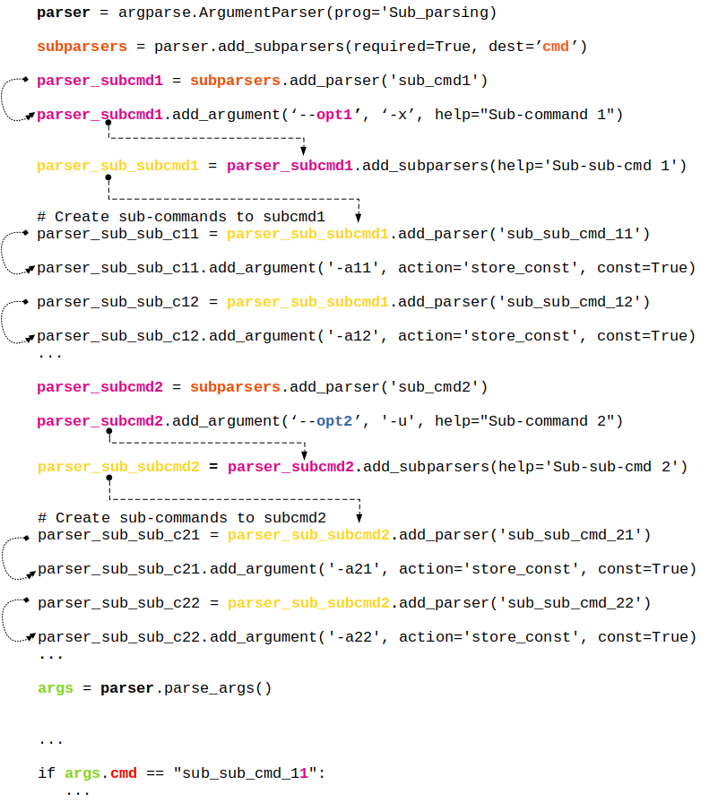
Summary of 'action' keyword
| Action Keyword | Action Performed by Argparser | Remark |
| store | This just stores the argument’s value | This is the default action |
| store_const | This stores the value specified by the const keyword which defaults to None. | Commonly used with optional arguments to specify some sort of flag |
| store_true | Special case of 'store_const' | To store the value True |
| store_false | Special case of 'store_const' | To store the value False |
| append | Stores a list, and appends each argument value to the list | It is useful to allow an option to be specified multiple times |
| append_const | Stores a list, and appends the value specified by the const keyword argument to the list | Useful when multiple arguments need to store constants to the same list |
| count | Counts the number of times a keyword argument occurs | For example, this is useful for increasing verbosity levels |
| help | Prints a complete help message for all the options in the current parser and then exits. | By default a help action is automatically added to the parser |
| version | Prints version information and exits when invoked | This expects a 'version=' keyword argument in the add_argument() call |
| extend | Stores a list, and extends each argument value to the list | Similar to 'append' |
The information tabulated above is just a re-formatting of text available at docs.python.org/3/library/argparse.html
Few Tips: re-organized from official documentation
- ArgumentParser, by default groups arguments into positional arguments and options when displaying help messages. add_argument_group() method can be used to group arguments as per user-defined category which displays arguments in separate groups in help messages.
- When parsers share a common set of arguments, the definitions of these arguments does not need to be repeated by using a single parser with all the shared arguments and passed to parents= argument to ArgumentParser. Such parent parsers must specify add_help=False to prevent conflicting help messages.
- To globally suppress attribute creation on parse_args() calls, parser = argparse.ArgumentParser( argument_default = argparse.SUPPRESS ).
- By default, for positional argument actions, the dest value is used directly, and for optional argument actions, the dest value is uppercased.
- metavar can be used to change the displayed name of an argument and a tuple can be provided to metavar to specify different display names for each of the arguments.
- As evident, hyphen '-' is used for positional arguments or can be used to specify a negative value to an argument. parse_args() method takes the convention: "positional arguments may only begin with - if they look like negative numbers and there are no options in the parser that look like negative numbers".
Linear algebra deals with system of linear algebraic equations where the coefficients of independent variables {x} are stored as a matrix [A] and the constant terms on the right hand side of equations are stored as a column vector {b}.
| Usage | OTAVE | Python (NumPy) |
| Array Index | 1-indexed | 0-indexed |
| Inverse of a square matrices (a 2D array in numPy) | inv(A) | inv(A) |
| Find the solution to the linear equation [A].{x} = {b} | x = linsolve (A, b) or x = A \ b or x = mldivide (A, b) | solve(A, b) |
| Eigen-values (V) and eigen vectors (λ): [A].{x} = λ{x} | [V, lambda] = eig (A) | eigvals(A): only eigen-values, eig(A): both eigen-values & eigen-vectors |
| Determinant of an array: product of singular values of the array | det(A) | det(A) |
| Generalized pseudo-inverse of A which is same as the inverse for invertible matrices | pinv(A, tol) | pinv(A) |
| The rank of a matrix is the number of linearly independent rows or columns and determines how many particular solutions exist to a system of equations. OCTAVE compute the rank of matrix A using the singular value decomposition. | ||
| Rank: number of singular values of A > specified tolerance tol | rank(A, tol) | (x, resids, rank, s) = lstsq (A, b, tol) |
| Cholesky decomposition, L of A such that A = LLH | chol(A, "lower") | cholesky (A): by default it computes lower triangular matrix |
Statistics
This topics includes basic descriptive statistics, probability distribution functions, hypothesis tests, design-of-experiments (DOE), random number generation ... Descriptive statistics refers to the methods to represent the essence of a large data set concisely such as the mean (average of all the values), median (the value dividing the dataset in two halves), mode (most frequently occurring value in a dataset), range (the difference between the maximum and the minimum of the input data)... functions which all summarize a data set with just a single number corresponding to the central tendency of the data.
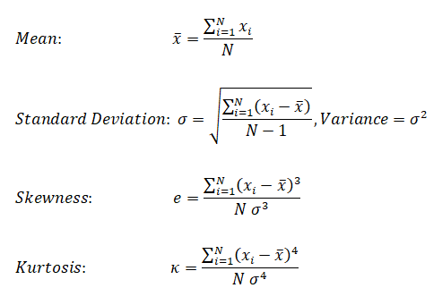
Median is the 50 percentile, the value that falls in the middle when the observations are sorted in ascending of descending order. While standard deviation is a measure of central tendency, skewness is the measure of assymetry (skew or bias in the data). Kurtosis is measure of deviation from normal distribution.
| Evaluation parameter | OTAVE | Python (numPy) |
| Mean (average) | mean(x) | mean(x) |
| Median (value that divides dataset) | median(x) | median(x) |
| Mode (most frequently occurring value) | mode(x) | mode(x) |
| Range | range(x) | ptp(x) |
| Mean of squares | meansq(x) | - |
| Variance | var(x) | var(x) |
| Standard deviation | std(x) | std(x) |
| Skewness | skewness(x) | skew(x)* |
| Kurtosis | kurtosis(x) | kurtosis(x)* |
| All-in-one | statistics (x) | describe(x) |
statistics(x): OCTAVE returns a vector with the minimum, first quartile, median, third quartile, maximum, mean, standard deviation, skewness, and kurtosis of the elements of the vector x.
Cheat-sheet: R-programming
- Get help on any specific named function, for example solve, use: help(solve). An alternative is: > ?solve
- R is an expression language and is case sensitive
- Commands are separated either by a semi-colon (‘;'), or by a newline. Elementary commands can be grouped together into one compound expression by braces ‘{' and ‘}'.
- Comments can be put almost anywhere, starting with a hashmark (‘#'), everything to the end of the line is a comment.
- If a command is not complete at the end of a line, R will give a different prompt, by default '+' on second and subsequent lines and continue to read input until the command is syntactically complete.
- If commands are stored in an external file, say commands.r in present working directory: source("commands.r")
- The function sink("record.list") will divert all subsequent output from the console to an external file, record.lis
- The command sink() restores it to the console once again
- Variable assignment is by either of 3 operators: equal operator '=', leftward operator "<-", rightward operator "->"
- Arrays: c() function which means to combine the elements into a vector. fruits <- c("banana", "apple", "mango"). In R - matrix is a two-dimensional rectangular data set, arrays can be of any number of dimensions set by dim attribute.
- Colon operator - Similar to OCTAVE, ':' creates a series of numbers in sequence for a vector. e.g. v <- 1:5 will create v = (1 2 3 4 5)
- Loops: the syntax for Loops in R is similar to that in C.
- Plots: the plot command in R is similar to that in OCTAVE or MATLAB - plot(x, y). Method to add color and title are different than OCTAVE: color = "green", main = "Chart Tile" is used to specify color of plot and title of the plot respectively.
- In OCTAVE, subplot(231) creates an array of 2x3 = 6 plots. The third digit specifies location of image in 2x3 matrix. In R, mfcol = c(3, 2) sets multiple figure environment and mfg = c(3, 2, 1, 1) specified position of the current figure in a multiple figure environment.
- Reading database
Following plots are generated in GNU OCTAVE script described later.
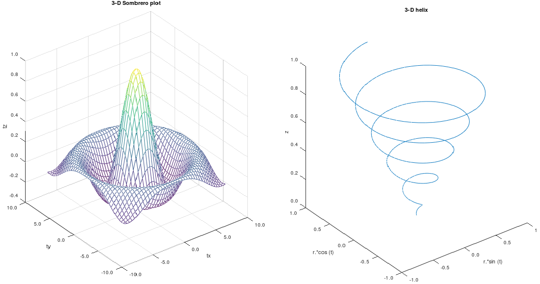
%Examples of 3D plots
%-------------------- -------------------------- ------------------------------
%  3D Somerero Plot
figure ();

subplot (1,2,1);
tx = ty = linspace(-8, 8, 41)';
[xx, yy] = meshgrid(tx, ty);
r = sqrt(xx .^ 2 + yy .^ 2) + eps;
tz = sin(r) ./ r;

mesh(tx, ty, tz);
xlabel("tx"); ylabel("ty"); zlabel("tz");
title("3-D Sombrero plot");

% Format X-, Y- and Z-axis ticks
xtick = get(gca,"xtick"); ytick = get(gca,"ytick");  ztick = get(gca,"ztick");
xticklabel = strsplit (sprintf ("%.1f\n", xtick), "\n", true);
set (gca, "xticklabel", xticklabel)
yticklabel = strsplit (sprintf ("%.1f\n", ytick), "\n", true);
set (gca, "yticklabel", yticklabel);
zticklabel = strsplit (sprintf ("%.1f\n", ztick), "\n", true);
set (gca, "zticklabel", zticklabel);
%-------------------- -------------------------- ------------------------------
%  3D Helix
subplot(1,2,2);
t = 0:0.1:10*pi;
r = linspace(0, 1, numel(t));  % numel(t) = number of elements in object 't'
z = linspace(0, 1, numel(t));
plot3(r.*sin(t), r.*cos(t), z);
xlabel("r.*sin (t)"); ylabel("r.*cos (t)"); zlabel("z");
title("3-D helix");

% Format X-, Y- and Z-axis ticks
xtick = get(gca,"xtick"); ytick = get(gca,"ytick");  ztick = get(gca,"ztick");
xticklabel = strsplit (sprintf ("%.1f\n", xtick), "\n", true);
set (gca, "xticklabel", xticklabel)
yticklabel = strsplit (sprintf ("%.1f\n", ytick), "\n", true);
set (gca, "yticklabel", yticklabel);
zticklabel = strsplit (sprintf ("%.1f\n", ztick), "\n", true);
The Python code to generate the 3D Helix is as follows.
import matplotlib as mpl; import matplotlib.pyplot as plt
from mpl_toolkits.mplot3d import Axes3D; import numpy as np
#-------------------- -------------------------- ------------------------------
mpl.rcParams['legend.fontsize'] = 10

fig = plt.figure(); ax = fig.gca(projection='3d')
t = np.linspace(0, 10 * np.pi, 100); r = np.linspace(0, 1, np.size(t));
z = np.linspace(0, 1, np.size(t));   x = r * np.sin(t); y = r * np.cos(t)

ax.plot(x, y, z, label='3D Helix');  ax.legend(); plt.show()
The Python code to generate the 3D Somerero Plot is as follows.
from mpl_toolkits.mplot3d import Axes3D; import numpy as np
import matplotlib.pyplot as plt; from matplotlib import cm
from matplotlib.ticker import LinearLocator, FormatStrFormatter

fig = plt.figure(); ax = fig.gca(projection='3d')

tx = np.arange(-8, 8, 1/40);  ty = np.arange(-8, 8, 1/40)
xx, yy = np.meshgrid(tx, ty); r = np.sqrt(xx**2 + yy**2)
tz = np.sin(r) / r
#-------------------- -------------------------- ------------------------------
# Plot the surface
sf = ax.plot_surface(xx,yy,tz, cmap=cm.coolwarm, linewidth=0, antialiased=False)

# Customize the z axis
ax.set_zlim(-1.01, 1.01); ax.zaxis.set_major_locator(LinearLocator(10))
ax.zaxis.set_major_formatter(FormatStrFormatter('%.02f'))

# Add a color bar which maps values to colors
fig.colorbar(sf, shrink=0.5, aspect=5); plt.show()
KNN is classified as non-parametric method because it does not make any assumption regarding the underlying data distribution. It is part of a "lazy learning technique" because it memorizes the data during training time and computes the distance during testing. It is part of algorithms known as Instance-based Algorithm as the method categorize new data points based on similarities to training data. This set of algorithms are sometimes also referred to as lazy learners because there is no training phase. Lack of training phase does not mean it is an unsupervised method, instead instance-based algorithms simply match new data with training data and categorize the new data points based on similarity to the training data.
#        KNN            K-Nearest-Neighbour    Python/scikit-learn
# ------------------------------------------------------------------------------
# Implement K-nearest neighbors (KNN) algorithm: supervised classfication method
# It is a non-parametric learning algorithm, which implies it does not assume
# any pattern (uniformity, Gaussian distribution ...) in training or test data
# --------------- STEP-1 ------------------------- -----------------------------
# Import libraries for maths, reading data and plotting
import numpy as np
import matplotlib.pyplot as plt   #from matplotlib import pyplot as plt
from matplotlib.colors import ListedColormap
import pandas as pd
from sklearn.model_selection import train_test_split
from sklearn.neighbors import NearestNeighbors
#Import classifier implementing the k-nearest neighbors vote.
from sklearn.neighbors import KNeighborsClassifier
#Import to evaluate the algorithm using confusion matrix
from sklearn.metrics import classification_report, confusion_matrix
# --------------- STEP-2 ------------------------ ------------------------------
# Import iris data, assign names to columns and read in Pandas dataframe
# url = "https://archive.ics.uci.edu/ml/machine-learning-databases/iris/iris.data"
header = ['sepal-length', 'sepal-width', 'petal-length', 'petal-width', 'Class']
dataset = pd.read_csv('iris.csv', names=header)

# Check content of dataset by print top 5 rows
# print(dataset.head())

A = dataset.iloc[:, :2].values    # Attributes = X
L = dataset.iloc[:, 4].values     # Labels = y

# Split the dataset into 75% training data and remainder as test data
A_trn, A_tst, L_trn, L_tst = train_test_split(A, L, test_size=0.25)
#test_size: if float, should be between 0.0 and 1.0 and represents proportion
#of the dataset to include in the test split. If int, represents the absolute
#number of test samples. If 'None', the value is set to the complement of the
#train size. If train_size is also 'None', it will be set to 0.25.

# ----------------STEP-3 -------------------------------------------------------
# Performs feature scaling
from sklearn.preprocessing import StandardScaler
scaler = StandardScaler()
scaler.fit(A_trn)
A_trn = scaler.transform(A_trn)
A_tst = scaler.transform(A_tst)

# ----------------STEP-4 -------------------------------------------------------
n_neighbors = 10
#initialize with a parameter: # of neighbors to use for kneighbors queries.
classifier = KNeighborsClassifier(n_neighbors, weights='uniform', algorithm='auto')
# algorithm = 'auto', 'ball_tree', 'kd_tree', 'brute'

#Fit the model using X [A_trn] as training data and y [L_trn] as target values
clf = classifier.fit(A_trn, L_trn)

#Make prediction on provided data [A_tst] (check test_size in train_test_split)
L_pred = classifier.predict(A_tst)

#Return probability estimates for the test data [A_tst]
print(classifier.predict_proba(A_tst))

#Return the mean accuracy on the given test data and labels.
print("\nClassifier Score:")
print(classifier.score(A_tst, L_tst, sample_weight=None))

#Compute confusion matrix to evaluate the accuracy of a classification. By
#definition a confusion matrix C is such that Cij is equal to the number of
#observations known to be in group 'i' but predicted to be in group 'j'. Thus
# in binary classification, the count of true negatives is C(0,0), false
#negatives is C(1,0), true positives is C(1,1) and false positives is C(0,1).
print("\n Confusion matrix:")
print(confusion_matrix(L_tst, L_pred))

#Print the text report showing the main classification metrics
#L_tst: correct target values, L_pred: estimated targets returned by classifier
print(classification_report(L_tst, L_pred))

# ----------------STEP-5 ------------------------ ------------------------------
# Calculating error for some K values, note initialization value was 5
error = []
n1 = 2
n2 = 10
for i in range(n1, n2):
    knn = KNeighborsClassifier(n_neighbors=i)
    knn.fit(A_trn, L_trn)
    pred_i = knn.predict(A_tst)
    error.append(np.mean(pred_i != L_tst))

#Plot the error values against K values
plt.figure(figsize=(8, 5))
plt.plot(range(n1, n2), error, color='red', linestyle='dashed', marker='o',
  markerfacecolor='blue', markersize=10)
plt.title('Error Rate K Value')
plt.xlabel('K Value')
plt.ylabel('Mean Error')

# ----------------STEP-6 ---------------------------- --------------------------
h = 0.025  #Step size in x-y grid
clf = classifier.fit(A, L)
# Create color maps
cmap_light = ListedColormap(['#009688', '#E0F2F1', 'violet'])
cmap_bold = ListedColormap(['#FF0000', '#00FF00', '#0000FF'])

# Plot the decision boundary and assign a color to each point in the mesh
# [x1, x2]x[y1, y2].
x1, x2 = A[:, 0].min() - 1, A[:, 0].max() + 1
y1, y2 = A[:, 1].min() - 1, A[:, 1].max() + 1
xx, yy = np.meshgrid(np.arange(x1, x2, h), np.arange(y1, y2, h))
Z = clf.predict(np.c_[xx.ravel(), yy.ravel()])

# Put the result into a color plot
Z = Z.reshape(xx.shape)
plt.figure()

plt.pcolormesh(xx, yy, Z, cmap=cmap_light)
# Plot also the training points
plt.scatter(A[:, 0], A[:, 1], c=L, cmap=cmap_bold, edgecolor='k', s=20)
plt.xlim(xx.min(), xx.max())
plt.ylim(yy.min(), yy.max())
plt.title("KNN (k = %i, weights = '%s')" %(n_neighbors, 'uniform'))

plt.show()                #pyplot doesn't show the plot by default
Outputs from this program are:
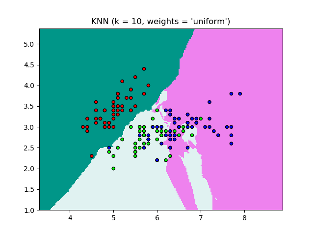
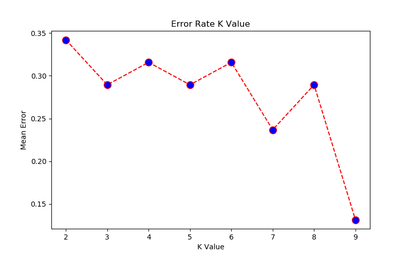
[x1, x2, x3 ... xm] are known values. [y1, y2 ... yp] are known labels. Equation of hyperplane is f(x) = xTβ + b = 0. Any classification task usually involves following steps:
- separate data into training and testing sets where each instance in the training set contains one target value or desired output (i.e. the class labels) and several attributes (i.e. the features or observed variables)
- produce a model (based only on the training data) which predicts the target values
- check the model on the test data given only the test data attributes
Support vector machines (SVM) were originally designed for binary (type-1 or type-2) classification. Some other methods known for multi-class classification are "one-against-all or one-vs-all", "one-against-one" and Directed Acyclic Graph Support Vector Machines (DAGSVM). SVM requires that each data set is represented as a vector of real numbers as shown below. Each column is known as class or category and each row is an observation (training data).
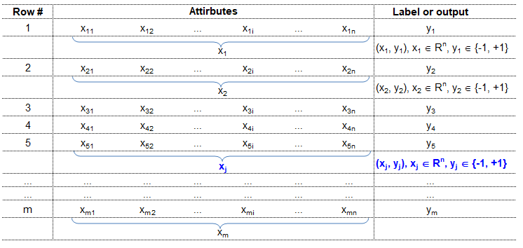
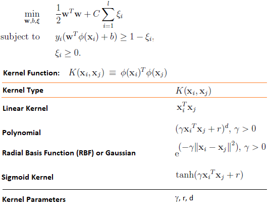
Reference: A Practical Guide to Support Vector Classfication by Chih-Wei Hsu, Chih-Chung Chang and Chih-Jen Lin, Department of Computer Science, National Taiwan University, Taipei 106, Taiwan
Scaling before applying SVM is very important. The main advantage of scaling is to avoid attributes in greater numeric ranges dominating those in smaller numeric ranges. Another advantage is to avoid numerical difficulties during the calculation. Because kernel values usually depend on the inner products of feature vectors, e.g. the linear kernel and the polynomial kernel, large attribute values might cause numerical problems. We recommend linearly scaling each attribute to the range [-1; +1] or [0; 1].
In general, the RBF kernel is a reasonable first choice. This kernel non-linearly maps samples into a higher dimensional space so it can handle the case when the relation between class labels and attributes is non-linear. If the number of features is large, one may not need to map data to a higher dimensional space. That is, the non-linear mapping does not improve the performance. Using the linear kernel is good enough, and one only searches for the parameter C.There are two parameters for an RBF kernel: C and γ. It is not known beforehand which C and γ are best for a given problem; consequently some kind of model selection (parameter search) must be done. The goal is to identify good (C, γ) so that the classifier can accurately predict unknown data (i.e. testing data). If the number of features is large, one may not need to map data to a higher dimensional space. That is, the non-linear mapping does not improve the performance. Using the linear kernel is good enough, and one only searches for the parameter C.
Support Vector Machines (clustering algorithm) tested for iris.data.
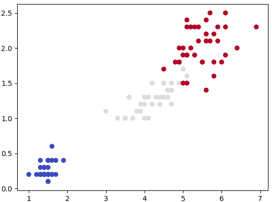
#        ssssssss       v           v       M            M
#        ss              v         v        M  M       M M
#        ss               v       v         M    M   M   M
#        ssssssss          v     v          M      M     M
#              ss           v   v           M            M
#              ss            v v            M            M
#        ssssssss             v             M            M
#
# SVM: "Support Vector Machine" (SVM) is a supervised ML algorithm which can be
#      used for both (multi-class) classification and/or (logistic) regression.
# Support vectors: vectors formed by observations w.r.t. origin
# Support Vector Machine is a separator which best segregates the two or more
# classes (hyperplanes or lines).

from sklearn import svm
import matplotlib.pyplot as plt
import numpy as np
import pandas as pd
#from sklearn import datasets     # Get pre-defined datasets e.g. iris dataset

# importing scikit learn with make_blobs
from sklearn.datasets.samples_generator import make_blobs

# creating datasets X containing n_samples, Y containing two classes
x, y = make_blobs(n_samples=500, centers=2, random_state=0, cluster_std=0.40)

#Generate scatter plot
#plt.scatter(x[:, 0], x[:, 1], c=y, s=50, cmap='spring')

'''
#------------------ Read the data ---------------------------------------------
dat = pd.read_csv("D:/Python/Abc.csv")
X = dat.drop('Class', axis=1)   #drop() method  drops the "Class" column
y = dat['Class']
'''
header=['sepal-length', 'sepal-width', 'petal-length', 'petal-width', 'Class']
df = pd.read_csv('iris.csv', names=header)
A = df.iloc[:, 2:4].values   # Use the last two features: note 2:4 slice
#To get columns C to E (unlike integer slicing, 'E' is included in the columns)
#df.loc[:, 'C':'E']

L = df.iloc[:, 4].values     # Labels: last column of input data

from sklearn.model_selection import train_test_split
X_trn, X_test, Y_trn, Y_test = train_test_split(A, L, test_size = 0.25)

#plt.scatter(x[:, 0], x[:, 1], c=y, s=50, cmap='spring')
plt.scatter(X_trn[:, 0], X_trn[:, 1], c=Y_trn, cmap=plt.cm.coolwarm)
plt.show()                         #By default, pyplot does not show the plots

#------------------ Specify SVM parameters ------------------------------------
# Specify penalty or regularization parameter 'C'
C = 1.0

# Carry out SVM calculation using kernel 'linear', 'rbf -  Gaussian kernel'
# 'poly', 'sigmoid'. Here rbf, poly -> non-linear hyper-planes
# rbf = Radial Basis Function Kernel
# gamma: Kernel coefficient for 'rbf', 'poly' and 'sigmoid'.
# Higher value of gamma tries to exact fit the training data -> over-fitting

# 'linear' -> classify linearly separable data
'''
from sklearn.svm import SVC
svcLin = SVC(kernel='linear', C=1, gamma='auto')
svcPoly = SVC(kernel='poly', degree=8)
svcc.fit(X_trn, Y_trn)
'''
# Following line of code is equivalent to the 3 short lines described above
svcLin1 = svm.SVC(kernel='linear', C=1.0, gamma='scale').fit(X_trn, Y_trn)
svcRBF = svm.SVC(kernel='rbf', C=1.0, gamma='scale').fit(X_trn, Y_trn)
svcPoly3 = svm.SVC(kernel='poly', C=1.0, degree=3).fit(X_trn, Y_trn)
svcLin2 = svm.LinearSVC(C=1.0, max_iter=10000).fit(X_trn, Y_trn)
# --------------- Create x-y grid to generate a plot --------------------------
#Calculate x- and y-limits
x_min, x_max = X_trn[:, 0].min() - 1, X_trn[:, 0].max() + 1
y_min, y_max = X_trn[:, 1].min() - 1, X_trn[:, 1].max() + 1
#Calculate grid size on x- and y-axis
h = (x_max - x_min)/100
xx, yy = np.meshgrid(np.arange(x_min, x_max, h), np.arange(y_min, y_max, h))

# ----------------- Generate the plot ------------------------------------------
# title for the plots
titles = ['SVC-No-Kernel', 'SVC-RBF', 'SVC-poly-3', 'LinearSVC']
for i, classifier in enumerate((svcLin1, svcRBF, svcPoly3, svcLin2)):
    # Plot the decision boundary and assign a color to each point
    plt.subplot(2, 2, i + 1)
    plt.subplots_adjust(wspace=0.4, hspace=0.4)

    #numpy.c_: Translates slice objects to concatenation along the second axis
    #numpy.ravel: returns a contiguous flattened array
    Z = classifier.predict(np.c_[xx.ravel(), yy.ravel()])

    #Put the result into a color plot
    Z = Z.reshape(xx.shape)
    plt.contourf(xx, yy, Z, cmap=plt.cm.gray, alpha=0.8)

    #Plot also the training points
    plt.scatter(X_trn[:,0], X_trn[:,1], c=Y_trn, facecolors='none', edgecolors='k')
    plt.xlabel('X1')
    plt.ylabel('X2')
    plt.xlim(xx.min(), xx.max())
    plt.ylim(yy.min(), yy.max())
    plt.xticks(())
    plt.yticks(())
    plt.title(titles[i])
plt.show()                        #By default, pyplot does not show the plots
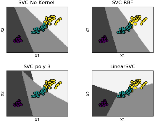
It is an unsupervised clustering algorithm where user needs to specify number of clusters - based on certain insights or even the "later purpose such as number of market segments". Though the number of clusters may not be known a-priori, a practically 'optimum' value can be estimated by "elbow method". It is a plot of cost function (grand total of distances between the cluster centroid and the observations) vs. number of clusters. Very often but not always, the curve looks like a "bent human hand" and the elbow represents the point where the curve has noticeable change in slope - the optimal value of 'K'.
- K-Means is also known as "hard clustering" technique where each input data point is associated with a unique cluster and thus lack flexibility in shape of clusters.
- There is no "probability function" or uncertainty associated with clustering to describe how close or appropriate this classification is.
- k-means inherently assumes that the cluster models must be circular and has no built-in way of accounting for oblong or elliptical clusters.
- Enhancements comes in the form of a GMM - Gaussian Mixture Model. Excerpt from scikit-learn: GMM is a probabilistic model that assumes all the data points are generated from a mixture of a finite number of Gaussian distributions with unknown parameters. This is a generalizing k-means clustering to incorporate information about the covariance structure of the data as well as the centers of the latent Gaussians.
- Thus, GMM is a 'soft' version of k-means.
# ----Ref: github.com/trekhleb/machine-learning-octave/tree/master/k-means-----
% K-means is an example of unsupervised learning, an iterative method over
% entire data. K-means is a clustering method and not classification method.
% Input is a set of unlabelled data and output from k-means is a set or sub-
% set of coherent data. It is not same as K-Nearest-Neighbours [KNN].
%
% Initialization
clear; close all; clc;

% ------------------------------ Clustering -----------------------------------
%Load the training data
load('set1.mat');

%Plot the data.
subplot(2, 2, 1);
plot(X(:, 1), X(:, 2), 'k+','LineWidth', 1, 'MarkerSize', 7);
title('Training Set');

%Train K-Means: The first step is to randomly initialize K centroids.
%Number of centroids: how many clusters are to be defined
K = 3;

%How many iterations needed to find optimal centroids positions 'mu'
max_iter = 100;
% Initialize some useful variables.
[m n] = size(X);

%Step-1: Generate random centroids based on training set. Randomly reorder the
%indices of examples: get a row vector containing a random permutation of 1:n
random_ids = randperm(size(X, 1));

% Take the first K randomly picked examples from training set as centroids
mu = X(random_ids(1:K), :);

%Run K-Means.
for i=1:max_iter
  % Step-2a: Find the closest mu for training examples.
  % Set m
  m = size(X, 1);

  % Set K
  K = size(mu, 1);

  % We need to return the following variables correctly.
  closest_centroids_ids = zeros(m, 1);

  %Go over every example, find its closest centroid, and store
  %the index inside closest_centroids_ids at the appropriate location.
  %Concretely, closest_centroids_ids(i) should contain the index of centroid
  %closest to example i. Hence, it should be a value in the range 1..K
  for i = 1:m
    d = zeros(K, 1);
    for j = 1:K
      d(j) = sum((X(i, :) - mu(j, :)) .^ 2);
    end
    [min_distance, mu_id] = min(d);
    closest_centroids_ids(i) = mu_id;
  end

  %Step-2b: Compute means based on closest centroids found in previous step
  [m n] = size(X);

  %Return the following variables correctly
  mu = zeros(K, n);

  %Go over every centroid and compute mean of all points that belong to it.
  %Concretely, the row vector centroids(i, :) should contain the mean of the
  %data points assigned to centroid i.
  for mu_id = 1:K
    mu(mu_id, :) = mean(X(closest_centroids_ids == mu_id, :));
  end
end

% Plotting clustered data
subplot(2, 2, 2);
for k=1:K
  % Plot the cluster - this is the input data marked as subsets or groups
  cluster_x = X(closest_centroids_ids == k, :);
  plot(cluster_x(:, 1), cluster_x(:, 2), '+');
  hold on;

  % Plot the centroid estimated by clustering algorithm
  centroid = mu(k, :);
  plot(centroid(:, 1), centroid(:, 2), 'ko', 'MarkerFaceColor', 'r');
  hold on;
end
title('Clustered Set');
hold off;
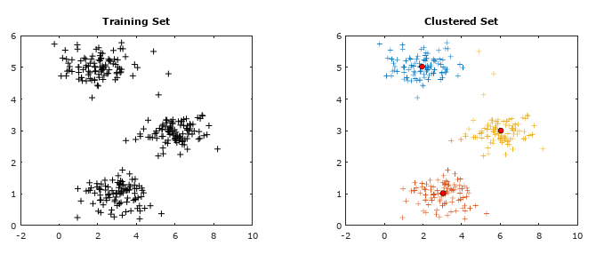
Machine Learning: Hierarchical Clustering
This type of clustering method is used on a relatively smaller datasets as the number of computation is proportional to N3 which is computationally expensive on big datasets and may not fit into memory.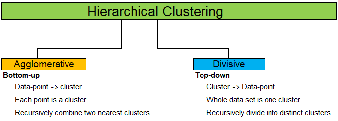
Random Forest Algorithm with Python and Scikit-Learn
Random Forest is a supervised method which can be used for regression and classification though it is mostly used for the later due to inherent limitations in the former. As a forest comprised of trees, a Random Forest method use multiple Decision Trees to arrive at the classification. Due to multiple trees, it is less prone to over-fitting and can handle relatively larger dataset having higher dimensionality (higher number of features). It is also known as Ensemble Machine Learning algorithm where many weak learning algorithms (the decision trees) are used to generate a majority vote (the stronger team). Bagging and boosting are two methods used in Random Forest learning algorithm to improve its performance: reduce bias and variance, increase accuracy.Bagging: bootstrap aggregation - where bootstring refers to training samples generated at random but with replacements. e.g. k samples out of N training data.Thus, the rows in each training samples may contain repeated values.
Boosting: it is an iterative approach by adjusting the probability of an instance to be part of subsequent training dataset if it is not correctly classified. The method starts with assigning equal probability to each instance to be part of first training set T1. The classifier C1 is trained on T1. It is then used to predict instances [xi, yi, i = 1, 2, 3 ... N]. If instances xm, xp and xz are not correctly classified, a higher probability will be assigned to these instances to be part on next training set T2. Since the selection of dataset is random, there are rows of dataset which may not make it to the any training set. They are known as out-of-bag dataset. A practically useful boosting algorithm is AdaBoost (which is a shorthand for Adaptive Boosting). The AdaBoost algorithm outputs a hypothesis that is a linear combination of simple hypotheses where an efficient weak learner is 'boosted' into an efficient strong learner.
Following example demonstrates use of Python and sciKit-Learn for classification. Problem Statement: The task here is to predict whether a person is likely to become diabetic or not based on four attributes: Glucose, Blood Pressure, BMI, Age.
The data in CSV format can be downloaded from here.import pandas as pd
import numpy as np
# --------- STEP-1: Read the dataset -------------------------------------------
dataset = pd.read_csv('diabetesRF.csv')
dataset.head()
X = dataset.iloc[:, 0:4].values
y = dataset.iloc[:, 4].values
# --------- STEP-2: Split the data into training and test sets -----------------
#Divide data into attributes and labels
from sklearn.model_selection import train_test_split
X_tr, X_ts, y_tr, y_ts = train_test_split(X, y, test_size=0.3, random_state=0)
#test_size: if float, should be between 0.0 and 1.0 and represents proportion
#of the dataset to include in the test split. If int, represents the absolute
#number of test samples. If 'None', the value is set to the complement of the
#train size. If train_size is also 'None', it will be set to 0.25.
# --------- STEP3: Scale the features ------------------------------------------
from sklearn.preprocessing import StandardScaler
sc = StandardScaler()
X_tr = sc.fit_transform(X_tr)
X_ts = sc.transform(X_ts)
# --------- STEP-4: Train the algorithm ----------------------------------------
from sklearn.ensemble import RandomForestClassifier
clf = RandomForestClassifier(n_estimators=20, random_state=0)
clf.fit(X_tr, y_tr)
y_pred = clf.predict(X_ts)
#
# --------- STEP-5: Evaluate the Algorithm -------------------------------------
from sklearn.metrics import classification_report, confusion_matrix
from sklearn.metrics import accuracy_score
#
#scikit-learn.org/stable/modules/generated/sklearn.metrics.confusion_matrix.html
#Compute confusion matrix to evaluate the accuracy of a classification. By
#definition a confusion matrix C is such that Cij is equal to the number of
#observations known to be in group 'i' but predicted to be in group 'j'. Thus
#in binary classification, the count of true negatives is C(0,0), false
#negatives is C(1,0), true positives is C(1,1) and false positives is C(0,1).
#
#In sciKit-learn: By definition, entry (i, j) in a confusion matrix is number of
#observations actually in group 'i', but predicted to be in group 'j'. Diagonal
#elements represent the number of points for which the predicted label is equal
#to the true label, while off-diagonal elements are those that are mislabeled by
#the classifier. Higher the diagonal values of the confusion matrix the better,
#indicating many correct predictions. i = 0, j = 0 -> TN, i = 0, j = 1 -> FP
#
print("Confusion Matrix as per sciKit-Learn")
print(" TN | FP ")
print("-------------------")
print(" FN | TP ")
print(confusion_matrix(y_ts,y_pred))
#
# Confusion matrix in other programs and examples
#
# Actual Values
# .----------------------,---------------------.
# P ! | !
# r Positives (1) ! True Positives (TP) | False Positives (FP)!
# e ! Predicted = Actual | (Type-1 Error) !
# d ! | !
# i !----------------------|---------------------!
# c ! | !
# t Negatives (0) ! False Negatives (FN)| True Negatives (TN) !
# e ! (Type-II Error) | Predicted = Actual !
# d ! | !
# Value !......................!.....................|
#
print("Classification Report format for BINARY classifications")
# P R F S
# Precision Recall fl-Score Support
# Negatives (0) TN/[TN+FN] TN/[TN+FP] 2RP/[R+P] size-0 = TN + FP
# Positives (1) TP/[TP+FP] TP/[TP+FN] 2RP/[R+P] size-1 = FN + TP
#
# F-Score = harmonic mean of precision and recall - also known as the Sorensen–
# Dice coefficient or Dice similarity coefficient (DSC).
# Support = class support size (number of elements in each class).
#
print(classification_report(y_ts, y_prd))
#
# Print accuracy of the classification = [TP + TN] / [TP+TN+FP+FN]
print("Classifier Accuracy = {0:8.4f}".format(accuracy_score(y_ts, y_prd)))
#
# --------- STEP-6: Refine the Algorithm ---------------------------------------
Recall: How many relevant items are selected?
Precision: How many selected items are relevant?
Decision Tree: This is a supervised classification method. Refer to the following decision making chart.
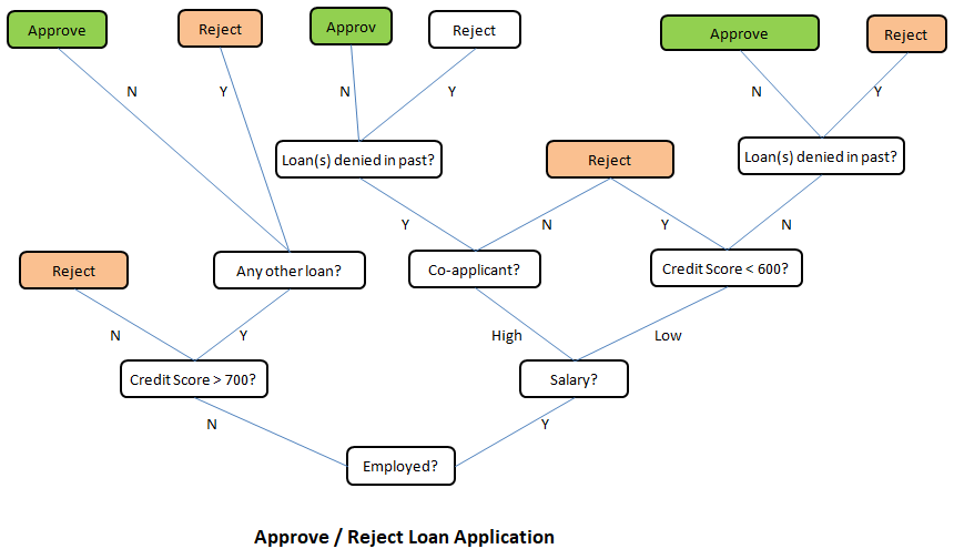

The method "decision tree" inherits this name from the structure of a 'tree' and the final intent to arrive at a 'decision' after going through a set of steps. As evident from the layout, the process starts with a "main node" known as "root node" and branches into other "leaf nodes" like a tree. In machine learning algorithms, following key points need to be addressed: Which attribute to select as root node? How to split attributes? When to stop? Before one gets to the answers, following concepts related to this machine learning methods needs to be understood:
- Entropy: This is a measure of impurity, uncertainty and information content. In thermodynamics and statistical mechanics, entropy is measure of disorder or randomness. In other words, entropy is a measure of lack of order. Entropy = Σ(-pi . log2pi). Entropy concepts have been adopted from information theory. The higher the entropy the more the information content or impurity.
- Information Gain: This is a measure of reduction in uncertainties and hence value lies between 0 and 1. Information gain tells us how important a given attribute of the feature vectors is and hence how useful it is for discriminating between the classes to be learned. Information gain = ENTROPYPARENT - average(ENTROPYCHILDREN).
- What is the entropy of a group in which all examples belong to the same class?
- A: pi = 1.0, Entropy = 0.0. This is not considered a good training set for learning.
- What is the entropy of a group with 50% in either class?
- A: pi = 0.5, Entropy = 1.0. This is considered a good training set for learning.
| Salaried | Married | Owns a house | Invests in Stocks? |
| Low | Y | 2BHK | 1 |
| Low | N | 2BHK | 1 |
| Low | Y | 3BHK | 0 |
| High | N | 3BHK | 0 |
p+ = fraction of positive examples = 2/4 = 0.5
p- = fraction of negative examples = 2/4 = 0.5
Thus: entropy of parent = Σ(-pi . log2pi) = -p+ log2(p+) - p- log2(p-) = 1.0.Split on feature 'Salaried'
| Salaried | Invests in Stocks? |
| Low | 1 |
| Low | 1 |
| Low | 0 |
| High | 0 |
Similarly, there is 1 instance of 'High' resulting in 1 negative label (class). p+,HIGH = 0. Hence, p-, HIGH = 1 - 0 = 1. Entropy at child node: EHIGH = -p+, HIGH log2(p+, HIGH) - p-, HIGH log2(p-, HIGH) = -0 × log2(0) - 1 × log2(1) = 0.
Information gain = EPARENT - pLOW × ELOW - pHIGH × EHIGH = 1.0 - 3/4 × (log23 - 2/3) - 1/4 × 0 = 1.5 - 3/4×log2(3) =0.3112.Split on feature 'Married'
| Married | Invests in Stocks? |
| Y | 1 |
| N | 1 |
| Y | 0 |
| N | 0 |
Similarly, there are 2 instances of 'N' resulting in 1 positive label (class) and 1 negative class. p+,N = 1/2. Hence, p-, N = 1.0 - 1/2 = 1/2. Entropy at child node: EN = -p+, N log2(p+, N) - p-, N log2(p-, N) = -1/2 × log2(1/2) - 1/2 × log2(1/2) = 1.0.
Information gain = EPARENT - pY × EY - pN × EN = 1.0 - 2/4 × 1.0 - 2/4 × 1.0 = 0.0.Split on feature "Owns a House"
| Owns a House | Invests in Stocks? |
| 2BHK | 1 |
| 2BHK | 1 |
| 3BHK | 0 |
| 3BHK | 0 |
Similarly, there are 2 instances of '3BHK' resulting in 2 negative label (class). p-,3HBK = 2/2 = 1.0. Hence, p+, 3BHK = 1.0 - 1.0 = 0.0. Entropy at child node: E3BHK = -p+, 3BHK log2(p+, 3BHK) - p-, 3BHK log2(p-, 3BHK) = -0.0 × log2(0.0) - 1.0 × log2(1.0) = 0.0.
Information gain = EPARENT - p2BHK × E2BHK - p3BHK × E3BHK = 1.0 - 2/4 × 0.0 - 2/4 × 0.0 = 1.0.Thus splitting on attribute (feature) "Owns a House" is best.
Probability in Machine Learning
Bayes theorem is a basis of a popular algorithm known as Naive Bayes Classification. This is widely used in text filtering such as classification of an e-mail as genuine or spam, categorization of a news article or user comment as fair or abusing / derogatory and the famous Monty Hall problem. However, it gets a bit complicated as the term 'odds' is also used to express the likelihood of an event - where 'odds' is not same as 'probability'. The odds of an event [E] vs. event "not E" or event [E'] are the ratio of their probabilities. For a standard dice, the odds of rolling digit 3 is [1/6] / [5/6] = 1:5, that the odds are "1 to 5 for" or "5 to 1 against" rolling a 3. The adjective 'Naive' refers to the "Naive assumption" of conditional independence between every pair of a feature.Bayes theorem is based on conditional probability that is based on some background (prior) information. For example, every year approximately 75 districts in India faces drought situation. There are 725 districts in India. Thus, the probability that any randomly chosen district will face rain deficit in next year is 75/725 = 10.3%. This value when expressed as ratio will be termed prior odds. However, there are other geological factors that governs the rainfall and the chances of actual deficit in rainfall may be higher or lower than the national average.
Suppose section A of class 8 has 13 boys and 21 girls. Section B of the same class has 18 boys and 11 girls. You randomly calls a student by selecting a section randomly and it turns out to be a girl. What is the probability that the girl is from section A? Let:
- H = event that the student selected is from section 'A'
- G = event that the student selected is a 'girl'
- In terms of conditional probability (it is already known that the student picked is a girl), p(H|G) refers to the probability that the event 'H' occurred given that 'G' is known to have occurred. There is no straightforward way to estimate this value!
- However, it is very easy to calculate the the probability of student picked to be a girl if it is known that section chosen is A. That is, p(G|H) = 21/34.
- Bayes theorem is used to estimate p(H|G). Here p(H|G) = p(H)/p(G) × p(G|H). Thus, p(H/G) = [1/2] / [33/63] × 21/34 = 11/68.
- prior probability = p(H) = probability of the hypothesis before we see the data (girl being picked)
- posterior probability = p(H|G) = probability of the hypothesis (girl is from section A) after we see the data (girl is being picked) and the the value one is interested to compute.
- p(G|H) = probability of the data (girl) under the hypothesis (section A), called the likelihood.
In english translation, the meaning or synonyms of 'odds' are 'chances', 'probability', 'likelyhood'. However, 'odds' is distinguished from probability in the sense that the former is always a ratio of two integers where the later is a fraction which can be represented in %. By odds, for example 3:2 (three to 2), we convey that we expect that for every three cases of an outcome (such as a profitable trade), there are two cases of the opposite outcome (not a profitable trade). In other words, chances of a profitable trade are 3/[3+2] = 3/5 or probability of 60%.
If the metrological department of the country announces that it is 80% probability of a normal monsoon this year and it turns out to be a drought. Can we conclude that the weather forecast was wrong. No! The forecast said it is going to be a normal monsoon with 80% probability, which means it may turn out to be drought with 10% probability or 1 out of 5 years. This year turned out to be the 1 in 5 event. Can we conclude that the probability 80% was correct? No! By the same argument one could conclude that 75% chance of normal monsoon was also correct and both cannot be true at the same time.Likelihood ratio: The ratio used in example above (4 times higher chance of normal monsoon than not a normal monsoon) is called the likelihood ratio. In other words, likelihood ratio is the probability of the observation in case the event of interest (normal monsoon), divided by the probability of the observation in case of no event (drought). The Bayes rule for converting prior odds into posterior odds is:
posterior odds = likelihood ratio × prior odds or posterior odds = Bayes factor × prior odds.
- If "likelihood ratio" > 1, the posterior odds are greater than the prior odds and the data provides evidence in favour of hypothesis.
- If "likelihood ratio" < 1, the posterior odds are smaller than the prior odds and the data provides evidence against the hypothesis.
- If "likelihood ratio" = 1, the posterior odds are greater than the prior odds and the data provides evidence in favour of hypothesis.
Gaussian Naive Bayes on iris data using Python and scikit-learn
# --------------------------------- --------------------------------------------
# --- Gaussian Naive Bayes on IRIS data,  print confusion matrix as Heat Map ---

import numpy as np
import matplotlib
import matplotlib.pyplot as plt

#There are many built-in data sets. E.g. breast_cancer, iris flower type
#from sklearn.datasets import load_breast_cancer

#Load the iris dataset which is built into scikit-learn
from sklearn.datasets import load_iris
iris = load_iris()

#This object is  a dictionary and contains a description, features and targets:
#print(iris.keys())
#dict_keys(['target','target_names','data','feature_names','DESCR','filename'])

#Split matrix [iris] into feature matrix [X] and response vector {y}
X = iris.data           # X = iris['data'] - access data by key name
y = iris.target         # y = iris['target']

A = iris.target_names   # A = iris['target_names']
#print(A)
#['setosa' 'versicolor' 'virginica']

F = iris.feature_names  # F = iris['feature_names']
#print(F)
#['sepal length (cm)', 'sepal width (cm)', 'petal length (cm)', 'petal width (cm)']

L = np.array(['Label'])
#print(np.r_[[np.r_[F, L], np.c_[X, y]]])

#Split X and y into training and testing sets
from sklearn.model_selection import train_test_split
X_trn,X_test, y_trn,y_test = train_test_split(X,y, test_size=0.4,random_state=1)

#Train the model on training set
from sklearn.naive_bayes import GaussianNB
gnb = GaussianNB()
clf = gnb.fit(X_trn, y_trn)

#Make predictions on test data
y_pred = gnb.predict(X_test)

#Compare actual response values (y_test) with predicted response values (y_pred)
from sklearn import metrics
from sklearn.metrics import classification_report, confusion_matrix
from sklearn.metrics import accuracy_score

GNBmetric = metrics.accuracy_score(y_test, y_pred)*100
print("Gaussian Naive Bayes model accuracy (in %): {0:8.1f}".format(GNBmetric))

#2D list or array which defines the data to color code in Heat Map
XY = confusion_matrix(y_test, y_pred)
print(XY)

fig, ax = plt.subplots()
#The heatmap is an imshow plot with the labels set to categories defined by user
from matplotlib.colors import ListedColormap
clr = ListedColormap(['red', 'yellow', 'green'])
im = ax.imshow(XY, cmap=clr)

#Define tick marks which are just the ascending integer numbers
ax.set_xticks(np.arange(len(A)))
ax.set_yticks(np.arange(len(A)))

#Ticklabels are the labels to show - the target_names of iris data = vector {A}
ax.set_xticklabels(iris.target_names)
ax.set_yticklabels(iris.target_names)

#Rotate the tick labels and set their alignment.
plt.setp(ax.get_xticklabels(), rotation=45, ha="right", rotation_mode="anchor")

#Loop over the entries in confusion matrix [XY] and create text annotations
for i in range(len(A)):
    for j in range(len(A)):
        text = ax.text(j, i, XY[i, j], ha="center", va="center", color="w")

ax.set_title("Naive Bayes: Confusion Matrix as Heat Map")
fig.tight_layout()
plt.show()
This generates the following plot. 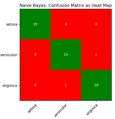
Monty-Hall Problem
Assume that in a TV show the candidate is given the choice between three doors. Behind two of the doors there is a pencil and behind one there is the grand prize, a car. The candidate chooses one door. After that, the show master opens another door behind which there is a pencil. Should the candidate switch doors after that? What is the probability of winning the car?Credibility of an Eyewitness
Assume that an eyewitness is 90% certain that a given person was involved in an accident. Moreover, assume that there were 20 people around the parking lot at the time of the crime. What is the posterior probability of the person actually have committed the crime?ANN: Artificial Neural Network
Multi-Layer Perceptron is a supervised learning algorithm which can learn a non-linear function approximator for either classification or regression. It differs from a logistic regression algorithm in construction where between the input and the output layer, there are one or more non-linear (hidden) layers. The simplest neural network consists of only one neuron and is called a perceptron. The perceptron is simply a witty name for the simple neuron model with the step activation function. A method for learning the weights of the perceptron from data called the Perceptron algorithm was introduced by the psychologist Frank Rosenblatt in 1957. It is just about as simple as the nearest neighbor classifier. The basic principle is to feed the network training data one example at a time. Each incorrect classification leads to an update in the weights and biases.In scikit-learn, MLP is implemented as following classes:
- MLPRegressor: this is a multi-layer perceptron (MLP) class that trains using back-propagation with no activation function in the output layer, which can also be seen as using the identity function as activation function. It uses the sum of square error (SSE) as the loss function and generates output as continuous values.
- MLPClassifier: a multi-layer perceptron (MLP) algorithm that trains using back-propagation that is using some form of gradient descent and the gradients are calculated using back-propagation.
- Many types of activation functions are available such as step function, sigmoid function, relu function and tanh function. In general, (rectified linear unit) ReLU function is used in the hidden layer neurons and sigmoid function is used for the output layer neuron.
Tensors
Tensors are a generalization of matrices. A constant or scalar is 0-dimensional tensor, a vector is a 1-dimensional tensor, a 2×2 matrix is a 2-dimensional tensor, a 3×3 matrix is a 3-dimensional tensor and so on. The fundamental data structure for neural networks are tensors. In summary, arrays, vectors, matrices and tensors are closely related concepts and differ only in the dimensions. All of these are a representation of a set of data with indices to locate and retrieve them.Steps to create a simple artificial neural network (ANN)
- Step-0: Read the data and manipulate it as per requirements of machine learning algorithms. For example, the labels may be categorical such as 'Rare', 'Low', 'Medium', 'High'. Neural networks (and most machine learning algorithms) work better with numerical data [0, 1, 2...]. Convert the categorical values to numerical values using LabelEncoder class from scikit-learn. Use y.Class.unique() to find unique categories in label vector.
- Step-1: Define the input layer, hidden layer(s) and the output layer. Chose activation function for every hidden layer - Sigmoid activation function is the most widely used one. Multi-layer Perceptron is sensitive to feature scaling, so it is highly recommended to scale the data - StandardScaler from scikit-learn can be used for standardization.
- Step-2: Feedforward or forward propagation: assumed weights [W] and biases [b] and calculate the predicted output y. Estimate accuracy of predictions using a Loss Function such as sum of squares error (SSE).
- Step-3: Back propagation: adjust weights and biases and calculate the predicted output y using gradient decent method which is based on derivative of the loss function with respect to the weights and biases.
- Step-4: Train the model
- Step-5: Test the model
# -------------------------------- ---------------------------------------------
# --- ANN - Multi-layer Perceptron,  print confusion matrix as Heat Map ---
import numpy as np
import matplotlib
import matplotlib.pyplot as plt

#There are many built-in data sets. E.g. breast_cancer, iris flower type
#from sklearn.datasets import load_breast_cancer
#df = load_breast_cancer()

#Load the iris dataset which is built into scikit-learn
from sklearn.datasets import load_iris
df = load_iris()

#This object is  a dictionary and contains a description, features and targets:
#print(df.keys())
#dict_keys(['target','target_names','data','feature_names','DESCR','filename'])

#Split matrix [df] into feature matrix [X] and response vector {y}
X = df.data           # X = df['data'] - access data by key name
y = df.target         # y = df['target']

A = df.target_names   # A = df['target_names']
#print(A)
#['setosa' 'versicolor' 'virginica']

F = df.feature_names  # F = df['feature_names']
#print(F)
#['sepal length (cm)', 'sepal width (cm)', 'petal length (cm)', 'petal width (cm)']

L = np.array(['Label'])
#print(np.r_[[np.r_[F, L], np.c_[X, y]]])

# splitting X and y into training and testing sets
from sklearn.model_selection import train_test_split
X_trn,X_test, y_trn,y_test = train_test_split(X,y, test_size=0.4,random_state=1)

#Scale or normalize the data
from sklearn.preprocessing import StandardScaler
#StandardScaler(copy=True, with_mean=True, with_std=True)
scaleDF = StandardScaler()
#Fit to the training data
scaleDF.fit(X_trn)
#Apply transformations to the data
X_trn = scaleDF.transform(X_trn)
X_test = scaleDF.transform(X_test)

#Train the model on training set
from sklearn.neural_network import MLPClassifier
ann_mlp = MLPClassifier(solver='lbfgs', alpha=1e-5,
                        hidden_layer_sizes=(5, 3), random_state=1)
clf = ann_mlp.fit(X_trn, y_trn)

#hidden_layer_sizes=(5, 3) - two layers having 5 and 3 nodes each
#max_iter = number of cycle of "feed-forward and back propagation" phase.

#Make predictions on the testing set
y_pred = ann_mlp.predict(X_test)

#Compare actual response (y_test) with predicted response (y_pred)
from sklearn import metrics
from sklearn.metrics import classification_report, confusion_matrix
from sklearn.metrics import accuracy_score

MLPmetric = metrics.accuracy_score(y_test, y_pred)*100
print("MLP accuracy(in %): {0:8.1f}".format(MLPmetric))

#2D list or array which defines the data to color code in Heat Map
XY = confusion_matrix(y_test, y_pred)
print(XY)
print(classification_report(y_test, y_pred))

fig, ax = plt.subplots()
#The heatmap is an imshow plot with the labels set to categories defined by user
from matplotlib.colors import ListedColormap
clr = ListedColormap(['grey', 'yellow', 'green'])
im = ax.imshow(XY, cmap=clr)

#Define the tick marks which are just the ascending integer numbers
ax.set_xticks(np.arange(len(A)))
ax.set_yticks(np.arange(len(A)))

#ticklabels are the labels to show - the target_names of iris data = vector {A}
ax.set_xticklabels(df.target_names)
ax.set_yticklabels(df.target_names)

#Rotate the tick labels and set their alignment.
plt.setp(ax.get_xticklabels(), rotation=45, ha="right", rotation_mode="anchor")

#Loop over the entries in confusion matrix [XY] and create text annotations
for i in range(len(A)):
    for j in range(len(A)):
        text = ax.text(j, i, XY[i, j], ha="center", va="center", color="w")

ax.set_title("ANN - Multi-layer Perceptron: Confusion Matrix")
fig.tight_layout()
plt.show()
Output of the program - MLP accuracy(in %): 70.0. Note that the lesser accuracy generated by the program does not highlight any deficiency in the algorithm or solver. This is only to show that there is no unique way of chosing the ANN parameters and optimal values need to be worked out by trial-and-error.
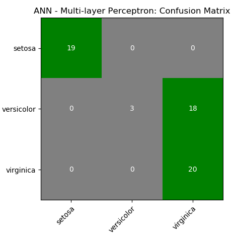
CNN
Convolutional Neural Networks (ConvNet or CNN) are special type of neural networks that handle image understanding and classification tasks by operating directly on the pixel intensities of input images. Thus, there is no need to explicitly perform any feature extraction operation.Digit Recognition
Excerpts from MathWorks Inc: "Object classification is an important task in many computer vision applications, including surveillance, automotive safety, and image retrieval. For example, in an automotive safety application, you may need to classify nearby objects as pedestrians or vehicles." The hand-written characters come in various shapes, size and colour. The correct classification of digits is one of the key aspects or capabilities of any ANN algorithm. This section describes the ANN implemented in MATLAB or GNU OCTAVE. The process starts with a dataset of digits (MNIST database or any similar ones) stored in this CSV file in Zip format.The information contained therein can be visualized using following script.
% ------ Handwritten digits classification ------------------------------------
%clear;
close all; clc;
colormap(gray);  % Use gray image colourmap
%
% Every row in X is a squared image reshaped into vector, width of each image
% is square root of total number of columns - 1 . The last column represents
% the actual digit hidden in those pictures. There are 500 examples each of 0,
% 1, 2, 3 ... 9.

A = csvread("digits.csv");
X =  A(:, 1:end-1);          %All columns except last one are pixels
Y = A(:, end);               %Last column has labels: 10 for digit '0'

% Randomly select N data points: required to split the dataset into training
% and test data. If N > 1, it is number. If it is a fraction, it is % of total
N_trn = 3000;
%
m = size(X, 1);        %Number of rows of X = no. of digits stored in  dataset
n = size(X, 2);        %Number of columns of X
nP = round(sqrt(n));   %Number of pixels rows,columns to represent each digit

% First row:
%   * * * * *  @ @ @ @ @  # # # # #      ```      $ $ $ $ $  [1 x n] vector
%
%   * * * * *
%   @ @ @ @ @
%   # # # # #
%      ...
%   $ $ $ $ $
%   D(1) = [nP x nP] matrix

% Second row:
%   * * * * *  @ @ @ @ @  # # # # #      ```      $ $ $ $ $  [1 x n] vector
%
%   * * * * *
%   @ @ @ @ @
%   # # # # #
%      ...
%   $ $ $ $ $
%   D(2) = [nP x nP] matrix

%Set padding: gap (shown as black background) between two consecutive images
pad = 2; ii = 25; jj = 20;
iR = pad + ii * (nP + pad);
iC = pad + jj * (nP + pad);
digit = -ones(iR, iC);

for s = 1: 10
% Copy each example into a [nP x nP] square block in the display array digit()
for i = 1:ii
 k = (i-1)*jj + 1 + (s-1)*ii*jj;
 for j = 1:jj
  % Get the max value of current row
  max_val = max(abs(X(k, :)));

  dR = pad + (i - 1) * (nP + pad) + (1:nP);
  dC = pad + (j - 1) * (nP + pad) + (1:nP);

  digit(dR, dC) = reshape(X(k, :), nP, nP) / max_val;
  k = k + 1;
 end
end

%imagesc(img) = display a scaled version of the matrix 'img' as a color image
%Colormap is scaled so that entries of the matrix occupy the entire colormap.
h = imagesc(digit, [-1 1]);    % Display Image
axis image off;        % Do not show axes

% Update figure windows and their children. Only figures that are modified
% will be updated. The refresh function can also be used to cause an update of
% the current figure, even if it is not modified.
drawnow;
str = sprintf(num2str(s-1));
saveas(h, str, 'png');

end
Rasterize and Vectorize: these are two frequently occuring terms in image handling programs. 'Rasterize' refers to converting an objects / images into pixels (though it is counter-intuitive as images are stored as pixels). Vectorization is a process of converting pixel information into geometry or outline information. The difference can be easily understood when texts are stored as 'non-selectable' images in a PDF (raster form) and same text are stored as 'selectable' objects in a PDF document (vector form).
Raster images lose quality when scaled up, resulting in pixelation (stair-stepping) and blurriness. Vector graphics consist of geometric shapes such as Bezier curves, B-splines, NURBS, arcs and lines determined by mathematical equations. Vector images can be significantly scaled without losing quality and hence such graphics are most appropriate for logos, icons, maps, graphs, illustrations... Vector images often result in smaller file sizes than raster images. Glyph Conversion is the method where tools like MS-Word translates the text characters into their corresponding visual glyphs (the shapes of the letters) based on font type. This makes the display theoretically "infinitely scalable". As the same time, it is counter-intuitive to think that when computer displays consists of finite number of pixels, how texts in MS-Word can be zoomed 'infinitely' without any stair-stepping? In real-life, one cannot draw a curve with smooth edge using small squares of uniform and finite size?
The images generated for digits 0, 3, 5 and 8 are shown below. The images for digit '1', digit '2', digit '3', digit '4', digit '5', digit '6', digit '7', digit '8' and digit '9' are under the respective hyperlinks.
% ------ Handwritten digits classification -------------------------------------
clear; close all; clc;

%Load training data, display randomly selected 100 data: X is the input matrix
load('digits.mat');
[m n] = size(X);   %Matrix [5000, 400], 1-500: 0, 501-1000: 1, 1001-1500: 2....

%Create random permutation: a column vector of size = size of input [X]
random_digits_indices = randperm(m);

%Select first 100 entries from the random permutation generated earlier
random_digits_indices = random_digits_indices(1:100);

%Display the 100 images stored in 100 rows as [10x10] layout of digits
%display_data(X(random_digits_indices, :));

% Setup the parameters you will use for this part of the exercise
% Specify number of input images of digits.
nD = 30;
input_layer_size = nD*nD;

% 1 <= Number of labels of digits =< 10, (note "0" mapped to label 10)
num_labels = 10;

fprintf('Training One-vs-All Logistic Regression...\n')
lambda = 0.01;
n_iter = 50;  %try 50, 100, 200 and check training set accuracy

% Train the model and predict theta [q] - the label 0 to 9
[all_theta] = one_vs_all_train(X, y, num_labels, lambda, n_iter);

fprintf('Predict for One-Vs-All...\n')
[iR iC] = size(X);
accu = ones(num_labels, 1);
for i = 1: num_labels
  if (i == 10)
   pred = one_vs_all_predict(all_theta, X(1:500, :));
   accu(i) = mean(double(pred == y(1:500))) * 100;
   fprintf('\n Training accuracy for digit 0 = %5.2f [%%]\n', accu(i));
  else
   j = i * iR/10 + 1;
   k = (i+1) * iR/10;
   pred = one_vs_all_predict(all_theta, X(j:k, :));
   accu(i) = mean(double(pred == y(j:k))) * 100;
   fprintf('\n Training accuracy for digit %d = %5.2f [%%]', i, accu(i));
  endif
end
%pred = one_vs_all_predict(all_theta, X);
fprintf('\n Overall training accuracy for all digits: %5.2f [%%]\n', mean(accu));
Output:
Training One-vs-All Logistic Regression...
Iteration    50 | Cost: 1.308000e-02
Iteration    50 | Cost: 5.430655e-02
Iteration    50 | Cost: 6.180966e-02
Iteration    50 | Cost: 3.590961e-02
Iteration    50 | Cost: 5.840313e-02
Iteration    50 | Cost: 1.669806e-02
Iteration    50 | Cost: 3.502962e-02
Iteration    50 | Cost: 8.498925e-02
Iteration    50 | Cost: 8.042173e-02
Iteration    50 | Cost: 6.046901e-03
Predict for One-Vs-All...

Training accuracy for digit 1 = 98.40 [%]
Training accuracy for digit 2 = 93.20 [%]
Training accuracy for digit 3 = 91.80 [%]
Training accuracy for digit 4 = 96.00 [%]
Training accuracy for digit 5 = 91.80 [%]
Training accuracy for digit 6 = 98.40 [%]
Training accuracy for digit 7 = 95.20 [%]
Training accuracy for digit 8 = 92.40 [%]
Training accuracy for digit 9 = 92.60 [%]
Training accuracy for digit 0 = 99.80 [%]

Oaverall training accuracy for all digits: 94.96 [%]
%-------------- FUNCTION: one_vs_all_train --------------------------------
% Trains logistic regression model each of which recognizes specific number
% starting from 0 to 9. Trains multiple logistic regression classifiers and
% returns all the classifiers in a matrix all_theta, where the i-th row of
% all_theta corresponds to the classifier for label i.

function [all_theta] = one_vs_all_train(X, y, num_labels, lambda, num_iter)

  [m n] = size(X);
  all_theta = zeros(num_labels, n + 1);

  % Add column of ones to the X data matrix.
  X = [ones(m, 1) X];

  for class_index = 1:num_labels
   % Convert scalar y to vector with related bit being set to 1.
   y_vector = (y == class_index);

   % Set options for fminunc
   options = optimset('GradObj', 'on', 'MaxIter', num_iter);

   % Set initial thetas to zeros.
   q0 = zeros(n + 1, 1);

   % Train the model for current class.
   gradient_function = @(t) gradient_callback(X, y_vector, t, lambda);

   [theta] = fmincg(gradient_function, q0, options);

   % Add theta for current class to the list of thetas.
   theta = theta';
   all_theta(class_index, :) = theta;
  end
end
% ------ Testing: Make predictions with new images ----------------------------
% Predicts the digit based on one-vs-all logistic regression approach.
% Predict the label for a trained one-vs-all classifier. The labels
% are in the range 1..K, where K = size(all_theta, 1)
function p = one_vs_all_predict(all_theta, X)
  m = size(X, 1); num_labels = size(all_theta, 1);

  % We need to return the following variables correctly.
  p = zeros(m, 1);

  % Add ones to the X data matrix
  X = [ones(m, 1) X];

  % Calculate probabilities of each number for each input example.
  % Each row relates to the input image and each column is a probability that
  % this example is 1 or 2 or 3...
  z = X * all_theta';
  h = 1 ./ (1 + exp(-z));

  %Now let's find the highest predicted probability for each row: 'p_val'.
  %Also find out the row index 'p' with highest probability since the index
  %is the number we're trying to predict. The MAX utility is describe below.

  %For a vector argument, return the maximum value.  For a matrix argument,
  %return a row vector with the maximum value of each column. max (max (X))
  %returns the largest element of the 2-D matrix X.  If the optional third
  %argument DIM is present then operate along this dimension.  In this case
  %the second argument is ignored and should be set to the empty matrix. If
  %called with one input and two output arguments, 'max' also returns the
  %first index of the maximum value(s).  [x, ix] = max ([1, 3, 5, 2, 5])
  %  x = 5, ix = 3

  [p_vals, p] = max(h, [], 2);
end
Limitations of this script in its current format and structure:
- Any input image has to be in a row format of size [1 x 400] only.
- The image has to be in grayscale and exactly of size 20px × 20px only
- The intensities of pixels must be supplied as signed double precision numbers.
- The background of images has to be dark (black) or gray only with font in white colour. The images with white background and black font will not get recognized.
- The scale of pixel intensities has no unique upper and lower bounds. In the entire dataset, the lowest and the highest values are -0.13196 and 10.0 respectively.
%Predict one digit at a time: digit from new set
fprintf('-----------------------------------------------------------------\n');
digit = 5; filename = [num2str(digit), ".png"];
dgt = rgb2gray(imread(filename));
Z = vec(im2double(dgt), 2);
%vec: return vector obtained by stacking the columns of the matrix X one above
%other. Without dim this is equivalent to X(:). If dim is supplied, dimensions
%of Z are set to dim with all elements along last dimension. This is equivalent
% to shiftdim(X(:), 1-dim).

pred = one_vs_all_predict(all_theta, Z);
fprintf('\nInput digit = %d, predicted digit = %d \n', digit, pred);
Input digit = 1, predicted digit = 5
Input digit = 3, predicted digit = 3Input digit = 4, predicted digit = 4
Input digit = 5, predicted digit = 3%------------------------------------------------------------------------------
Running the program repeatedly, correct prediction for digit 5 was obtained. However, the prediction for digit 1 remained as 5!
Further improvisation is possible by writing the answer on the right hand side or bottom of the image. Image is a matrix indexed by row and column values. The plotting system is, however, based on the traditional (x y) system. To minimize the difference between the two systems Octave places the origin of the coordinate system in the point corresponding to the pixel at (1; 1). So, to plot points given by row and column values on top of an image, one should simply call plot with the column values as the first argument and the row values as the second argument.%----------------- Example of PLOT over an IMAGE ------------------------------
I = rand (20, 20); %Generate a 2D matrix of random numbers
[nR, nC] = find (I > 0.95); %Find intensities greater than 0.95
hold ("on"); imshow (I); %Show image
plot(nC,nR,"ro"); hold ("off"); %Plot over the image
The output will look like: 
Digit Classification in Python
# --- Random Forest Classifier for Hand-written Digits ---

import matplotlib.pyplot as plt
from sklearn.datasets import load_digits
import pylab as pl

#Load hand-written digits from scikit-learn built-in database
digits = load_digits()

#Use a grayscale image
#pl.gray()
#pl.matshow(digits.images[0])
#pl.show()
#Check how digits are stored
print("Total digits in dataset are ", len(digits.images))

#Visualize few images in n x n matrix
n = 10
df = list(zip(digits.images, digits.target))
plt.figure(figsize = [5, 5])
for index, (image, label) in enumerate(df[:n*n]):
    plt.subplot(n, n, index+1)
    plt.axis('off')
    plt.imshow(image, cmap=plt.cm.gray_r, interpolation='nearest')
    #plt.title('%i' % label)
plt.show()

import random
from sklearn import ensemble, metrics
from sklearn.metrics import classification_report, confusion_matrix
from sklearn.metrics import accuracy_score

#Find out the number of digits, store label as variable y
nTest = len(digits.images)
x = digits.images.reshape(nTest, -1)
y = digits.target

#Create random indices to select training images, f = training set fraction
#The method used here is a longer version of train_test_split utility in sklearn
f = 0.20
idxTrain = random.sample(range(len(x)), round(len(x) * f))
idxTest = [i for i in range(len(x)) if i not in idxTrain]

#Sample and validation images
imgTrain = [x[i] for i in idxTrain]
imgTest = [x[i] for i in idxTest]

#Sample and validation targets
yTrain = [y[i] for i in idxTrain]
yTest = [y[i] for i in idxTest]

#Call random forest classifier
clf = ensemble.RandomForestClassifier(n_estimators=20, random_state=0)

#Fit model with training data
clf.fit(imgTrain, yTrain)

#Test classifier using validation images
score = clf.score(imgTest, yTest)
print("Random Forest Classifier: trained on ", len(imgTrain), "samples")
print("Score = {0:8.4f}". format(score))
#
yPred = clf.predict(imgTest)
XY = confusion_matrix(yTest, yPred)
print(XY)
Outputs from this Python code are:
Total digits in dataset are  1797
Random Forest Classifier: trained on  359 samples
Score =   0.9075
[[138   0   0   0   2   0   1   0   1   0]
 [  0 134   0   1   0   1   0   0   1   5]
 [  1   3 127   6   1   0   1   0   3   1]
 [  0   1   5 127   0   0   0   2  10   3]
 [  3   2   0   0 141   1   1   4   0   0]
 [  1   0   0   3   0 128   1   1   0   5]
 [  1   1   0   0   2   0 141   0   0   0]
 [  0   0   0   0   1   1   0 136   1   0]
 [  0   9   3   2   0   2   2   3 117   0]
 [  0   2   0   7   2   5   1  12   5 116]]
CBIR: Content Based Image Retrieval systems: method to find similar images to a query image among an image dataset. Example CBIR system is the search of similar images in Google search. Convolutional denoising autoencoder [feed forward neural network] - class of unsupervised deep learning.
Markov Chain and Hidden Markov Models (HMM)
As per MathWorks Inc: Markov processes are examples of stochastic processes - processes that generate random sequences of outcomes or states according to certain probabilities.
Also known as "time series analysis", this model is in many aspects similar to Naive-Bayes model and in fact based on Bayes theorem. HMM is used to find a likely sequence of events for a given sequence of observations. Here the probability of a future event is estimated based on relative frequency of past observations of sequence of events (thus known prior probabilities). Probabilities to go from state 'i' to state 'i+1' is known as transition probability. The emission probability refers to the likelihood of of a certain observation 'y' when model is in state 's'.Markov Chain: P(En|En-1, En-1 ... E2, E1) = probability of nth event given known outcome of past (n-1) events.
First Order Markov Assumption: P(En|En-1, En-1 ... E2, E1) = P(En|En-1) that is probability of nth event depends only of known outcome of previous event. This is also known as "memoryless process" because the next state depends only on the current state and not on the chain of events that preceded it or led the latest state. This is similar to tossing a fair coin. Even if one gets 5 or 20 successive heads, the probability of getting a head in next toss is still 0.50.
Markov first order assumption may or may not be valid depending upon the application. For example, it may not be a valid assumption in weather forecasting and movement of stock price. However, it can be a valid assumption in prediction of on-time arrival of a train or a flight.
Trellis Diagram: This is a graphical representation of likelihood calculations of HMMs.
Example calculations:
- Suppose the initial or prior probabilities of 'clear' and 'foggy' day during December-January in northern part of India are: P(C) = 0.3, P(F) = 0.7.
- The transition probabilities are: P(C|C) = 0.2, P(C|F) = 0.1, P(F|F) = 0.6, P(F|C) = 0.5
- Probability of a sequence of states in this example say P({F, F, C, C}) = P(C|C) × P(C|F) × P(F|F) × P(F) = 0.2 × 0.1 × 0.6 × 0.7 = 0.0084
The following OCTAVE script implements a Gaussian model to detect anomalous examples in a given dataset. The Gaussian distribution is mathematically represented as follows. The data in a CSV file used for cross-validation can be downloaded from here.
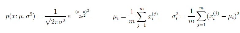
%----Ref: github.com/trekhleb/machine-learning-octave/anomaly-detection/--------
%Anomaly detection algorithm to detect anomalous behavior in server computers.
%The features measure the throughput (Mb/s) and latency (ms) of response of each
%server. m = 307 examples of how they were behaving, the unlabeled dataset. It
%is believed that majority of these data are normal or non-anomalous examples of
%the servers operating normally, but there might also be some examples of servers
%acting anomalously within this dataset. Label y = 1 corresponds to an anomalous
%example and y = 0 corresponds to a normal example.
clear; close all; clc;
%
%Load the data.
A = csvread("serverParams.csv");
X = [A(:, 1) A(:, 2)]; Y = A(:, 3);
%
%Estimate MEAN and VARIANCE: parameters of a Gaussian distribution
%Get number of training sets and features. size(X) returns a row vector with the
%size (number of elements) of each dimension for the object X. m=rows, n=cols
[m n] = size(X);
mu = mean(X);
s2 = (1 / m) * sum((X - mu) .^ 2);
%
%Visualize the fit
[X1, X2] = meshgrid(0 : 0.5 : 30);  U = [X1(:) X2(:)];
[m n] = size(U);
%
%Returns the density of the multivariate normal at each data point (row) of X
%Initialize probabilities matrix
Z = ones(m, 1);
%
%Go through all training examples and through all features. Returns the density
%of the multivariate normal at each data point (row) of X.
%
for i=1:m
  for j=1:n
    p = (1 / sqrt(2 * pi * s2(j))) * exp(-(U(i, j) - mu(j)) .^ 2 / (2 * s2(j)));
    Z(i) = Z(i) * p;
  end
end
Z = reshape(Z, size(X1));
%
%Visualize training data set.
plot(X(:, 1), X(:, 2),'bx'); hold on;
%
%Do not plot if there are infinities
if (sum(isinf(Z)) == 0)
  contour(X1, X2, Z, 10 .^ (-20:3:0)');
end
hold off;
xlabel('Latency (ms)'); ylabel('Throughput (MB/s)');
title('Anomaly Detection: Server Computers');
%
%Returns the density of the multivariate normal at each data point (row) of X
%Initialize probabilities matrix
[m n] = size(X); prob = ones(m, 1);
%
%Go through all training examples and through all features. Returns the density
%of the multivariate normal at each data point (row) of X.
for i=1:m
  for j=1:n
    p = (1 / sqrt(2 * pi * s2(j))) * exp(-(X(i, j) - mu(j)) .^ 2 / (2 * s2(j)));
    prob(i) = prob(i) * p;
  end
end
%
%Select best threshold. If an example x has a low probability p(x) < e, then it
%is considered to be an anomaly.
%
best_epsilon = 0;
best_F1 = 0;
F1 = 0;
ds = (max(prob) - min(prob)) / 1000;
prec = 0; rec = 0;
for eps = min(prob):ds:max(prob)
  predictions = (prob < eps);
  % The number of false positives: the ground truth label says it is not
  % an anomaly, but the algorithm incorrectly classifies it as an anomaly.
  fp = sum((predictions == 1) & (Y == 0));

  %Number of false negatives: the ground truth label says it is an anomaly, but
  %the algorithm incorrectly classifies it as not being anomalous.

  %Use equality test between a vector and a single number: vectorized way rather
  %than looping over all the examples.
  fn = sum((predictions == 0) & (Y == 1));

  %Number of true positives: the ground truth label says it is an anomaly and
  %the algorithm correctly classifies it as an anomaly.
  tp = sum((predictions == 1) & (Y == 1));

  %Precision: total "correctly predicted " positives / total "predicted" positives
  if (tp + fp) > 0
    prec = tp / (tp + fp);
  end
  %Recall: total "correctly predicted" positives / total "actual" positives
  if (tp + fn) > 0
    rec = tp / (tp + fn);
  end
  %F1: harmonic mean of precision and recall
  if (prec + rec) > 0
    F1 = 2 * prec * rec / (prec + rec);
  end

  if (F1 > best_F1)
    best_F1 = F1;
    best_epsilon = eps;
  end
end

fprintf('Best epsilon using Cross-validation: %.4e\n', best_epsilon);
fprintf('Best F1 on Cross-validation set:  %.4f\n', best_F1);

%Find the outliers in the training set and plot them.
outliers = find(prob < best_epsilon);

%Draw a red circle around those outliers
hold on
plot(X(outliers, 1), X(outliers, 2), 'ro', 'LineWidth', 2, 'MarkerSize', 10);
legend('Training set', 'Gaussian contour', 'Anomalies');
hold off
The output from the program is: 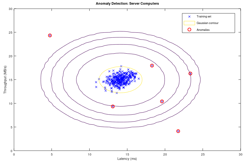
Recommender Systems and Collaborative Filtering
Collaborative filtering refers to the fact that contribution by each user by providing ratings to a product, book, music, brand, movie... etc help make a better rating system and in turn get a accurate rating for the product, brand, movie... for himself / herself. Users with ratings similar to a specific user 'A' is called neighbours of 'A'. All the ratings given by the user 'A' is called a "rating vector".Jaccard Similarity: similarity(A, B) = |rA ∪ rB| / |rA ∩ rB| where rA and rB are rating vectors for users A and B respectively. Thus: similarity(A, B) = total common ratings / total cumulative ratings. It ignores the rating values and is based solely on number of ratings by the users.
Cosine Similarity: similarity(A, B) = cos(rA, rB) which is similar to the dot product of vectors. Thus: similarity(A, B) = Σ[rA(i).rB(i)] / |rA| / |rA|. It treats the blank entries (missing values) in rating vector as zero which is counter-intuitive. If a user did not rate a product does not mean he/she strongly dislikes it.
Centred Cosine Similarity: This is very much similar to cosine similarity and is also known as Pearson Correlation. However, the rating vector for each user is "normalized about mean". Thus, r'A(i) = rA - [Σ(rA(i)]/N. similarity(A, B) = cos(r'A, r'B). It still treats the blank entries (missing values) in rating vector as zero which is average rating (note mean = 0). It handles the effect or bias introduced by "tough raters" and "easy raters" by normalizing their rating values.
Item-Item collaborative filtering refers to method of filtering based on ratings for items (books, movies...) by all users. User-User collaborative filtering refers to method of filtering based on all ratings by a user for items (books, music, movies...). Though both of these approach looks similar, the former performs significantly better than the later in most use cases. However, note that it is important to take care of user which has not rated any item than the item which has not got any rating. An item which has not been rated does not any way qualify for any recommendations to any user.Example: Given the rating for 8 movies by 9 users, estimate the rating of movie 'B' by user '3'.
| Movies | Users and their ratings | Rating vector | ||||||||
| 1 | 2 | 3 | 4 | 5 | 6 | 7 | 8 | 9 | ||
| A | 3.0 | 4.0 | 1.0 | 2.0 | 3.0 | 5.0 | rA | |||
| B | 2.0 | ? | 2.0 | 3.0 | 4.0 | rB | ||||
| C | 4.0 | 4.0 | 1.0 | 3.0 | 2.0 | rC | ||||
| D | 2.0 | 3.5 | 4.0 | 3.0 | 4.0 | rD | ||||
| E | 3.0 | 2.0 | 5.0 | 5.0 | 1.0 | 3.5 | rE | |||
| F | 2.0 | 1.0 | 4.0 | 3.0 | 5.0 | rF | ||||
| G | 1.0 | 2.0 | 3.0 | 4.0 | 2.0 | rG | ||||
| H | 1.0 | 2.0 | 3.0 | 2.0 | 5.0 | rH | ||||
Step-1: Normalize the ratings about mean zero and calculate centred cosine. In MS-Excel, one can use sumproduct function to calculate the dot product of two rows and columns. Thus: rA . rB = sumproduct(A1:A9, B1:B9) / sqrt(sumproduct(A1:A9, A1:A9)) / sqrt(sumproduct(B1:B9, B1:B9)).
| User | Users and their ratings after mean normalization | s(X, B): X = {A, B, C ... H} | ||||||||
| 1 | 2 | 3 | 4 | 5 | 6 | 7 | 8 | 9 | ||
| A | 0.000 | 1.000 | -2.000 | -1.000 | 0.000 | 2.000 | 0.000 | |||
| B | -0.750 | ? | -0.750 | 0.250 | 1.250 | 1.000 | ||||
| C | 1.200 | 1.200 | -1.800 | 0.200 | -0.800 | 0.012 | ||||
| D | -1.300 | 0.200 | 0.700 | -0.300 | 0.700 | 0.162 | ||||
| E | -0.250 | -1.250 | 1.750 | 1.750 | -2.250 | 0.250 | -0.063 | |||
| F | -1.000 | -2.000 | 1.000 | 0.000 | 2.000 | 0.048 | ||||
| G | -1.400 | -0.400 | 0.600 | 1.600 | -0.400 | -0.026 | ||||
| H | -1.600 | -0.600 | 0.400 | -0.600 | 2.400 | 0.328 | ||||
Step-2: For assumed neighbourhood of 3, find the 3 movies which has been rated by user 'B' and similarity s(X,B) is the highest in s(X,B) vector. Thus, movie A, D and H which are rated by user '3' and their similarities are highest among s(X,B).
Step-3: Use similarity weights and calculate weighted average. Similarity weights: s(C,B) = 0.012, s(D,B) = 0.162, s(H,B) = 0.328. Likely rating of movie by user '3' = weighted average calculated as follows.
r(B, 3) = s(C,B) . r(C,3) + s(D,B) . r(D,3) + s(H,B) . r(H,3) / [s(C,B) + s(D,B) + s(H,B)] = (0.012 * 4.0 + 0.162 * 3.5 + 0.328 * 2.0) /(0.012 + 0.162 + 0.328) = 2.53
The following code is an improvisation of GNU OCTAVE script available on gitHub. There are many versions of this scripts uploaded there. The movie rating data in CSV (zip) format can be downloaded from here. Other functions are available here: fmincg.m, collaborative filtering coefficients and movie id / name. This script is for demonstration only and not fully debugged: the predicted rating is higher than 5 which is not correct.
% -----------------------Movie Recommender using GNU OCTAVE / MATLAB -----------
clc; clear;
%
%Load data from a CSV file: first half contains rating and later half ON/OFF key
A = csvread("movieRatings.csv");
[m2, n] =  size(A); m = m2 / 2;
%
%Split the matrix A into user rating matrix 'Y' and  1/0 matrix 'R'
Y = A([1:m], :); R = A([m+1:m2], :);
%
%Find out no. of non-zero elements (actual number of ratings) in each row
Yc = sum(Y ~= 0, 2);
fprintf('\nHighest number of ratings received for a movie: %d \n', max(Yc));
%
% Read the movie list
fid = fopen('movie_ids.txt');
g = textscan(fid,'%s','delimiter','\n');  n = length(g{1}); frewind(fid);
movieList = cell(n, 1);
for i = 1:n
  line = fgets(fid); % Read line
  [idx, mName] = strtok(line, ' '); %Word Index (ignored since it will be = i)
  movieList{i} = strtrim(mName);   % Actual Word
end
fclose(fid);
%
%Initialize new user ratings
ratings = zeros(1682, 1);
%
%return
%Stop execution and return to command prompt - useful for debugging
%
% Y = 1682x943 matrix, containing ratings (1-5) of 1682 movies by 943 users
% R = 1682x943 matrix, where R(i,j) = 1 if user j gave a rating to movie i
% q(j) = parameter vector for user j
% x(i) = feature vector for movie i
% m(j) = number of movies rated by user j
% tr(q(j)) * x(i) = predicted rating for user j and movie i
%
fprintf('\n Training collaborative filtering...\n');
%
%Estimate mean rating ignoring zero (no rating) cells
Ym = sum(Y, 2) ./ sum(Y ~=0, 2);
%
%Mean normalization
Yn = Y - Ym .* (Y ~= 0);
%
%mean(A,2) is a column vector containing the mean of each row
%mean(A) a row vector containing mean of each column
%
%Get data size
n_users    = size(Y, 2);
n_movies   = size(Y, 1);
n_features = 10;         %e.g. Romance, comedy, action, drama, scifi...
ratings    = zeros(n_users, 1);
%
%Collaborative filtering algorithm
%Step-1: Initialize X and Q to small random values
X = randn(n_movies, n_features);
Q = randn(n_users, n_features);    %Note Q (THETA) and q (theta) are different
q0 = [X(:); Q(:)];
%
%Set options for fmincg
opt = optimset('GradObj', 'on', 'MaxIter', 100);
%
%Set regularization parameter
%Note that a low value of lambda such as L = 10 results in predicted rating > 5.
% However, a very high value say L=100 results in high ratings for those movies
% which have received only few ratings even just 1 or 2.
L = 8;
q = fmincg (@(t)(coFiCoFu(t, Yn, R, n_users, n_movies, n_features, L)), q0,opt);
%
% Unfold the returned theta matrix [q] back into X and Q
X = reshape(q(1 : n_movies * n_features), n_movies, n_features);
Q = reshape(q(n_movies * n_features + 1:end), n_users, n_features);
%
fprintf('Recommender system learning completed.\n');

%Make recommendations by computing the predictions matrix.
p = X * Q';
pred = p(:,1) + Ym;
%
[r, ix] = sort(pred, 'descend');
fprintf('\n Top rated movies:\n');
for i=1:10
  j = ix(i);
  fprintf('Predicting rating %.1f for %s, actual rating %.2f out of %d\n', ...
    pred(j), movieList{j}, Ym(j), Yc(j));
end
Reinforcement Learning - RL
It is behavioral learning model which differs from other types of supervised learning methods because the system is not trained with the any labelled data set. This is a training algorithm based on 'rewards' and 'penalties' of an action. Like a child when on falls over a slippery (wet) surface, next time when someone has to cross such surface, he/she will use his/her toes to improve the grip and increase grip as the smoothness of the surface is felt. In RL, the terms agent, environment, reward, penalty and policy are most frequently used concepts. While in an organization, policy refers to a set of guidelines, templates, forms and workflows, in RL policy is a deep neural network (NN) which decides actions taken by the agent. The gaming program AlphaGo is based on RL algorithm. It can be applied in motion controls of a robotic arms to grasp and move items.While training a robot to balance itself while walking and running, the RL training algorithm cannot let it fall and learn, not only this method will damage the robot, it has to be picked and set upright every time it falls. Reinforcement learning is also the algorithm that is being used for self-driving cars. One of the quicker ways to think about reinforcement learning is the way animals are trained to take actions based on rewards and penalties. Do you know how an elephant is trained for his acts in a circus?
Q-Learning algorithm: this is based on Bellman equation [Q(s,a) = sT.W.a], where {s} is states vector, {a} denotes actions vector and [W] is a matrix that is learned] which calculates "expected future rewards" for given current state. The associated data is Q-table which is a 2D table with 'states' and 'actions' as two axes.Natural Language Processing (NLP)
Adapted from "Machine Learning For Dummies, IBM Limited Edition": NLP is the ability to train computers to understand both (hand-written and typed) text and human speech (voice). NLP techniques are needed to capture the meaning of unstructured text from documents or communication from the user. Therefore, NLP is the primary way that systems can interpret text and spoken language. NLP is also one of the fundamental technologies that allows non-technical people to interact with advanced technologies. For example, rather than needing to code, NLP can help users ask a system questions about complex data sets. Similarly, a user can develop his own website without knowing much about HTML and css. Unlike structured database information that relies on schemas to add context and meaning to the data, unstructured information must be parsed and tagged to find the meaning of the text. Tools required for NLP include categorization, ontologies, tapping, catalogues, dictionaries and language models.Model Selection Criteria
As evident in methods and programs outlined above, machine learning is about "selection of models and parameters". Field of information theory is used to quantify or measure the expected value of information - various goodness-of-fit tests have been developed to assess the performance of a model with respect to how well it explains the data. Akaike information criterion (AIC) is considered the first model selection criterion that is appropriate to be used in practice where the best model is the candidate model with the smallest AIC.Another criterion, the Bayesian information criterion (BIC) was proposed by Schwarz (also referred to as the Schwarz Information Criterion - SIC or Schwarz Bayesian Information Criterion - SBIC). This is a model selection criterion based on information theory which is set within a Bayesian context. Similar to AIC, the best model is the one that provides the minimum BIC. [Reference: www.methodology.psu.edu/resources/aic-vs-bic] AIC is better in situations when a false negative finding would be considered more misleading than a false positive. BIC is better in situations where a false positive is as misleading as or more misleading than a false negative.
One of the method to validate a model is known as "k-fold cross validation" which can be described as shown in following image.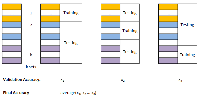
AI - The Unknown Beast!
AI has already started affecting my decisions and impulses. When I search for a flight ticket, related ads start appearing. I believe that fare starts increasing when I make many searches before actually booking and Uber or Ola cab. On the hindsight, so far none of the ads which pop-up through Google ads have helped me because they appear when I have already made the purchase or have pushed the buying decision for future months. Also, most of the ads appear not when I am interested to buy them but want to understand the technology behind them. Based on my browsing history and interest, the accuracy of ads shown by google is not more than 5%.I have certainly used the recommendations generated by youTube and viewed many videos based on their recommendations. Though I found them useful, there was nothing extra-ordinary in those recommendations.
One of the possible problem I see is the integrity and authenticity of data/information. I have come across many videos on youTube which are either too repetitive or fake or even factually incorrect. I have heard how AI can diagnose the disease from X-rays and CT-scans. In my opinion, an expert or experience doctor can identify the issue from naked eyes within seconds. These tools are going to make even a naive doctor look like expert! Hence, the AI may help incompetent doctors. How this capability is going to address the patient remains unanswered - will it lead to lesser consultation fee and/or lesser waiting time?
AI tools can also be considered having implications similar to "dynamite and laser". These are used for constructive purposes such as mining and medical diagnosis whereas dangerous aspects like "bomb blasts and laser-guided missiles" are also known. Is AI going to make "forensic expert's" life easy or tough? Is it going to introduce significant biases in the virtually opaque implementations in customer segmentations?
Identity Theft: E-mail address hunting, Reverse image search, Social Media post scraping, whois service of a website: reveals complete information (phone number, e-mail ID, residential address) if privacy protection is not enabled or purchased. OSINT: Open Source INTelligence is a way to gathering information from social media using usernames.
In the name of company policy, none of the social media platform publish (and shall publish) even a partial list of rules used by them to filter and delete/ban posts on their websites. This complete opaque implementation of AI tools is a lethal weapon to mobilize resources to affect public opinion and influence democratic processes. There are posts and videos on YouTube that threaten about annihilation of particular community. There are videos still up (as in Dec-2022) where a preacher claims Right of Islam to kill non-muslims and especially few special categories of non-muslims. However, the AI tool is configured such that anybody posting against that video content with same level of pushback (such as non-muslims also have right to kill muslims) shall get suspended from the platform. I firmly believe that any expectation that AI can be used to make the communication balanced, open and honest is just a wishful thinking - AI has created potential to make it more biased and one-sided than traditional modes.
Deep Learning
Python, TensorFlow and Keras: TensorFlow derives its name from "operations on tensors" where a tensor is a multi-dimensional array. It contains deep learning libraries which include those from Keras.Pandas
Print each column name as rowfor col_name in DataFrame.columns.to_numpy(): print(col_name).
DataFrame                                <- = Table
   col_1 | col_2 | col_3 | ... | col_N   <- Column Labels or Series

0   v_11 |  v_12 |  v_13 | ... |  v_1N   <- DataFrame.loc[0] `] df.loc[0: 2]
1   v_21 |  v_22 |  v_23 | ... |  v_2N   <- DataFrame.loc[1]  ]   or
2   v_31 |  v_32 |  v_33 | ... |  v_3N   <- DataFrame.loc[2] _] df.loc[0,1,2]
.
.
.
Cursor AI
Tag line on official website: "The AI Code Editor". More from website: "Cursor lets you write code using instructions. Update entire classes or functions with a simple prompt. Cursor's agent mode completes tasks end to end. It does this quickly, while keeping programmers in the loop. We support all frontier coding models, including Claude Sonnet 4, OpenAI o3-pro, OpenAI GPT-4.1, Gemini 2.5 Pro, Claude Opus 4, and more."Thus, Cursor AI is a code editor that uses artificial intelligence models to help code writers with coding tasks such as code generation, smart rewrites, codebase queries and end-to-end task completion.
Optimization Methods and Algorithms
The optimization method involves finding minima or maxima of a variable or a set of variables. Most basic version of optimization method taught during engineering is finding the values at which differential becomes zero. In real-life, the relation between dependent and independent variables are neither simple nor continuous. A quick summary of optimization methods used in industry can be found below.Examples of optimization problem statements
- The Traveling Salesman Problem: This is a classic combinatorial optimization problem. Given a list of cities and the distances between them, the goal is to find the shortest possible route that visits every city exactly once and returns to the origin city.
- Vehicle Routing Problem: Similar to previous, but adds constraints like variable delivery times, specific vehicle capacities, and multiple vehicles.
- Bin Packing Problem: Items of varying sizes must be packed into a finite number of bins (like container ships or delivery trucks) to minimize the number of bins used. The problem has many applications, such as filling up containers, loading trucks with weight capacity constraints, creating file backups in storage media and technology mapping in VLSI circuit design.
Classical Optimization Methods
Linear Programming (LP): Used when relationships are linear. Non-linear Programming: Handles non-linear system behavior such as wind turbine power curve optimization. Mixed-Integer Programming: Combines discrete and continuous variables.Heuristic Methods
These are methods based on phenomena in nature. Some of the algorithms are Genetic Algorithms (wind farm layout optimization), Particle Swarm Optimization (Parameter tuning in solar and wind systems), Simulated Annealing (Mimics cooling process of metals which can be used for grid configuration optimization) and Ant Colony Optimization (Inspired by ant pathfinding which can be used for optimal power flow).Machine Learning–Based Optimization: Reinforcement Learning, Optimization based on Deep Learning which combines prediction with decision-making.
Multi-Objective Optimization such as Pareto optimization - to find the best trade-off between different streams say Cost, Emissions and Reliability
Stochastic Optimization: Uses probabilistic models for cases with high uncertainties such as renewable energy sources due to weather-dependence.
As per aws.amazon.com/blogs/machine-learning/using-genetic-algorithms-on-aws-for-optimization-problems: "GAs use concepts from evolution such as survival of the fittest, genetic crossover, and genetic mutation to solve problems. Rather than trying to create a single solution, those evolutionary concepts are applied to a population of different problem solutions, each of which is initially random. The population goes through a number of generations, literally evolving solutions through mechanisms like reproduction (crossover) and mutation. After a number of generations of evolution, the best solution found across all the generations is chosen as the final problem solution."
Typical JD for a Optimization Specialist
| Job Title | Optimization Specialist | Job Type | Full-time |
| Cost Center | CC01 | Section Name | SH01 |
| Job Code | CC01_SH01_OS | Reports To | Delivery Head |
| Work Location | Kolkata | Number of Openings | 1 |
| Minimum Experience (years) | 5.0 | Maximum Experience (years) | 8.0 |
| Education Qualification | B. Tech. | Engineering Discipline | Applied Maths, Computer Science |
| Description of role | Applied Maths and Optimization Specialist to design, develop, and implement mathematical models and optimization algorithms for solving complex business and engineering problems. The roles requires strong analytical skills, expertise in optimization techniques, and experience applying mathematical methods to real-world systems. | ||
| Responsibilities | Develop mathematical and optimization models for business and technical problems. Design and implement algorithms for Mixed Integer Programming (MIP), Nonlinear Optimization and Heuristic and Meta-heuristic Optimization. Collaborate with software development teams to integrate optimization engines into web applications and cloud platforms. Present analytical findings and recommendations to stakeholders and leadership teams. Research emerging optimization methodologies and industry best practices. | ||
| Technical Skills Required with % weight | (a) Experience deploying optimization services in cloud-native environments. - 25%, (b) Strong knowledge of Optimization theory, Numerical methods, Statistical modeling and Algorithm design - 25%, (c) Proficiency in programming languages such as Python and MATLAB - 25% and (d) Experience with optimization tools/frameworks Gurobi and SciPy Optimize - 25% | ||
| Domain Skills Required with % weight | (i) Software development lifecycle (SDLC) - 25%, (ii) Exposure to industries such as Energy, Wind Power, Electrical Networks - 25%, (iii) Familiarity with machine learning, Genetic Algorithm, Multi-objective Optimization and AI-based optimization methods - 50% | ||
| Keywords and Tool Names | Python, SQL, Pandas, NumPy, SciPy, Gurobi, AWS hosting, SCRUM | ||
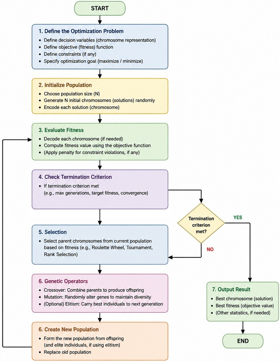
In optimization, a heuristic is a practical problem-solving method that seeks a good or near-optimal solution within a reasonable amount of time, rather than guaranteeing the mathematically optimal solution. Heuristics are particularly useful when: The search space is very large, exact optimization methods are computationally expensive, and a quick solution is more important than finding the absolute best solution. In short, heuristics are intelligent "rules of thumb" that guide the search toward good solutions when exact optimization is impractical or too expensive.
The problem to find a point which has shortest cumulative distance from a given set of point is the geometric median or L1-median or Euclidean minisum (also called the Fermat-Weber point). For such unconstrained problems, deterministic methods such as Weiszfeld's Algorithm are usually faster and more accurate, but the GA approach is useful when the problem needs to be extended with constraints, obstacles, weighted points, or additional optimization objectives. A sample code can be found here and the output generated is shown below.
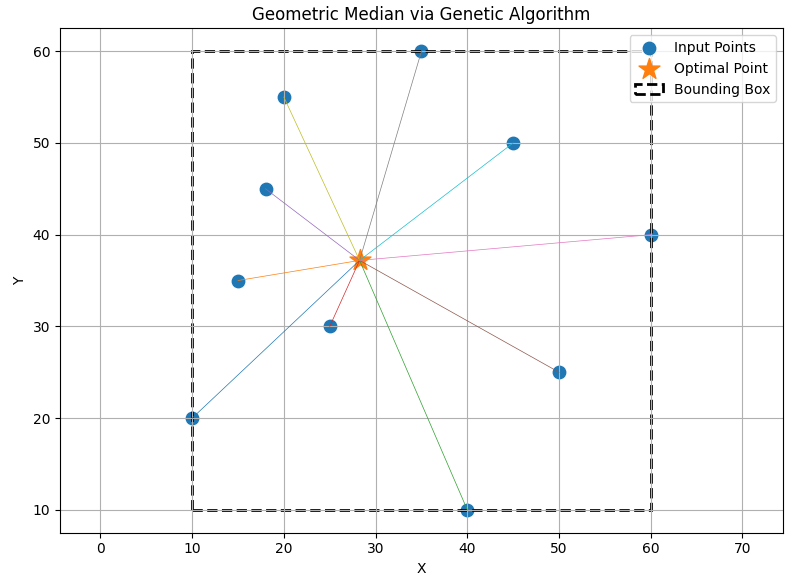
The content on CFDyna.com is being constantly refined and improvised with on-the-job experience, testing, and training. Examples might be simplified to improve insight into the physics and basic understanding. Linked pages, articles, references, and examples are constantly reviewed to reduce errors, but we cannot warrant full correctness of all content.
Template by OS Templates